Background
This example was developed by Julie Baniszewski, a PhD student in the Department of Entomology at Penn State. Julie participated in our last workshop in Mexico under the INTAD-Tag Along program (International Agriculture and Development graduate program). This is a robust example of using dose-response methods in R based on generalized linear modeling concepts (including mixed model).
Data set: Mosquito toxicity was tested with 4 instars and monitored until pupation. The experimental design was 3 blocks with 4 replicates each to test mosquito toxicity.
The aim is to look at ultimate %pupation and LC50, LC90 for 24, 48 hrs.
What is in the database? * Concentration = weight:volume concentration of chemical * Instar = 1-4 stages of mosquito larvae introduced to chemical treatment * Block = Growth Chamber * Rep = 1-4 replicates within each block * Total = total number of initial larvae * Pupae = total number of larvae that reached pupation * %Pupated = % larvae that pupated and ultimately survived the treatment * Day0 = total number of initial larvae * Day1p = proportion of larvae mortality on Day 1 post chemical exposure * Day2p = proportion of larvae mortality on Day 2 post chemical exposure
Load packages
Here, we will use the readxl package to work with Excel-oriented files. Like the nonparametric regression example, we have defined a local repository for the file and this can be changed for individual use. We have several other different packages specific to work with dose-response curves and model fitting.
library(readxl)
library(drc)
library(car)
library(cowplot)
library(tidyverse)
Importing data set:
DR <- read_excel("DR_Data_Sheet.xlsx")
str(DR)
## Classes 'tbl_df', 'tbl' and 'data.frame': 288 obs. of 22 variables:
## $ Concentration: num 0 0 0 0 1 1 1 1 0.75 0.75 ...
## $ Instar : num 1 1 1 1 1 1 1 1 1 1 ...
## $ Block : num 1 1 1 1 1 1 1 1 1 1 ...
## $ Rep : num 1 2 3 4 1 2 3 4 1 2 ...
## $ Total : num 10 11 10 10 10 10 10 10 10 10 ...
## $ Pupae : num 9 11 8 9 0 0 0 0 0 0 ...
## $ %Pupated : num 0.9 1 0.8 0.9 0 0 0 0 0 0 ...
## $ Day0 : num 10 11 10 10 10 10 10 10 10 10 ...
## $ Day1p : num 0.1 0 0.1 0.1 1 0.8 0.9 0.9 0.8 0.7 ...
## $ Day2p : num 0.1 0 0.1 0.1 1 1 1 1 1 0.9 ...
## $ Day3p : num 0.1 0 0.1 0.1 1 1 1 1 1 1 ...
## $ Day4p : num 0.1 0 0.1 0.1 1 1 1 1 1 1 ...
## $ Day5p : num 0.1 0 0.1 0.1 1 1 1 1 1 1 ...
## $ Day6p : num 0.1 0 0.1 0.1 1 1 1 1 1 1 ...
## $ Day7p : num 0.1 0 0.1 0.1 1 1 1 1 1 1 ...
## $ Day8p : num 0.1 0 0.1 0.1 1 1 1 1 1 1 ...
## $ Day9p : num 0.1 0 0.1 0.1 1 1 1 1 1 1 ...
## $ Day10p : num 0.1 0 0.1 0.1 1 1 1 1 1 1 ...
## $ Day11p : num 0.1 0 0.1 0.1 1 1 1 1 1 1 ...
## $ Day12p : num 0.1 0 0.1 0.1 1 1 1 1 1 1 ...
## $ Day13p : num 0.1 0 0.2 0.1 1 1 1 1 1 1 ...
## $ Day14p : num 0.1 0 0.2 0.1 1 1 1 1 1 1 ...summary(DR)## Concentration Instar Block Rep Total Pupae %Pupated Day0 Day1p Day2p Day3p Day4p Day5p Day6p Day7p Day8p Day9p Day10p Day11p Day12p Day13p Day14p
## Min. :0.0000 Min. :1.00 Min. :1 Min. :1.00 Min. :10.00 Min. : 0.000 Min. :0.000 Min. :10.00 Min. :0.0000 Min. :0.0000 Min. :0.0000 Min. :0.00000 Min. :0.0000 Min. :0.0000 Min. :0.0000 Min. :0.0000 Min. :0.0000 Min. :0.0000 Min. :0.0000 Min. :0.0000 Min. :0.0000 Min. :0.0000
## 1st Qu.:0.1000 1st Qu.:1.75 1st Qu.:1 1st Qu.:1.75 1st Qu.:10.00 1st Qu.: 0.000 1st Qu.:0.000 1st Qu.:10.00 1st Qu.:0.0000 1st Qu.:0.0000 1st Qu.:0.0000 1st Qu.:0.08333 1st Qu.:0.1000 1st Qu.:0.1000 1st Qu.:0.1000 1st Qu.:0.1000 1st Qu.:0.1000 1st Qu.:0.1000 1st Qu.:0.1404 1st Qu.:0.1404 1st Qu.:0.4000 1st Qu.:0.4000
## Median :0.3750 Median :2.50 Median :2 Median :2.50 Median :10.00 Median : 0.000 Median :0.000 Median :10.00 Median :0.3000 Median :0.6500 Median :0.7500 Median :0.80000 Median :0.8500 Median :0.9000 Median :0.9000 Median :1.0000 Median :1.0000 Median :1.0000 Median :1.0000 Median :1.0000 Median :1.0000 Median :1.0000
## Mean :0.4333 Mean :2.50 Mean :2 Mean :2.50 Mean :10.17 Mean : 3.615 Mean :0.346 Mean :10.17 Mean :0.3924 Mean :0.5186 Mean :0.5499 Mean :0.56945 Mean :0.5846 Mean :0.6026 Mean :0.6179 Mean :0.6258 Mean :0.6367 Mean :0.6425 Mean :0.6745 Mean :0.6778 Mean :0.7434 Mean :0.7454
## 3rd Qu.:0.7500 3rd Qu.:3.25 3rd Qu.:3 3rd Qu.:3.25 3rd Qu.:10.00 3rd Qu.: 9.000 3rd Qu.:0.900 3rd Qu.:10.00 3rd Qu.:0.8000 3rd Qu.:1.0000 3rd Qu.:1.0000 3rd Qu.:1.00000 3rd Qu.:1.0000 3rd Qu.:1.0000 3rd Qu.:1.0000 3rd Qu.:1.0000 3rd Qu.:1.0000 3rd Qu.:1.0000 3rd Qu.:1.0000 3rd Qu.:1.0000 3rd Qu.:1.0000 3rd Qu.:1.0000
## Max. :1.0000 Max. :4.00 Max. :3 Max. :4.00 Max. :14.00 Max. :14.000 Max. :1.000 Max. :14.00 Max. :1.0000 Max. :1.0000 Max. :1.0000 Max. :1.00000 Max. :1.0000 Max. :1.0000 Max. :1.0000 Max. :1.0000 Max. :1.0000 Max. :1.0000 Max. :1.0000 Max. :1.0000 Max. :1.0000 Max. :1.0000Preliminary examination of data
Start by looking at data (ultimate survival): dependent variable ‘%pupation’
op <- par(mfrow = c(1, 2), mar=c(3.2,3.2,2,.5), mgp=c(2,.7,0)) #make two plots in two columns
plot(DR$`%Pupated` ~ DR$Concentration, data = DR, main="Original Dose Scale")
plot(DR$`%Pupated` ~ logit(DR$Concentration+0.01), data = DR, main="Logarithmic Dose Scale")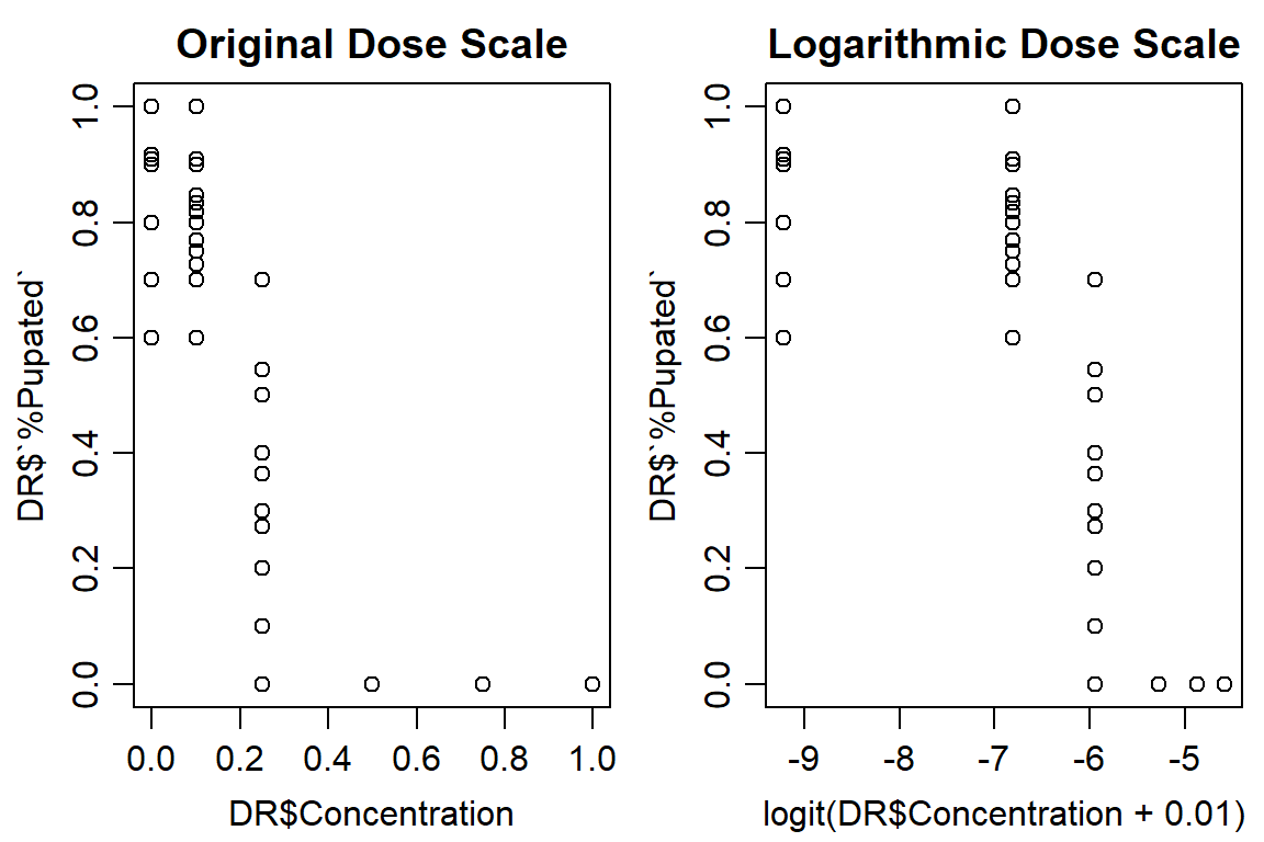
Look at control data
#if mortality is >> 5%, may need Abbot's Formula for correction (Correction%= (1-treatmetn/control)*100)

aggregate(DR[,7], list(DR$Concentration), mean)
## Group.1 %Pupated
## 1 0.00 0.9429293
## 2 0.10 0.9127889
## 3 0.25 0.2204545
## 4 0.50 0.0000000
## 5 0.75 0.0000000
## 6 1.00 0.0000000#Control is ~5% motality, is okayInitial models: dose-response and linear
Option 1: use Dose Response Model
DR1<-drm(DR$`%Pupated` ~ log1p(DR$Concentration), DR$Instar, data = DR, fct=LL.2(names=c("Slope", "LD50")), type=("binomial"), na.action=na.omit)
summary(DR1)
##
## Model fitted: Log-logistic (ED50 as parameter) with lower limit at 0 and upper limit at 1 (2 parms)
##
## Parameter estimates:
##
## Estimate Std. Error t-value p-value
## Slope:1 5.281684 1.480907 3.5665 0.0003618 ***
## Slope:2 4.639606 1.259559 3.6835 0.0002300 ***
## Slope:3 5.063119 1.466544 3.4524 0.0005556 ***
## Slope:4 4.753037 1.414136 3.3611 0.0007764 ***
## LD50:1 0.148070 0.019217 7.7050 1.309e-14 ***
## LD50:2 0.147669 0.019483 7.5795 3.466e-14 ***
## LD50:3 0.167355 0.021347 7.8398 4.477e-15 ***
## LD50:4 0.193382 0.023076 8.3800 < 2.2e-16 ***
## ---
## Signif. codes: 0 '***' 0.001 '**' 0.01 '*' 0.05 '.' 0.1 ' ' 1#look at residuals
op <- par(mfrow = c(1, 2), mar=c(3.2,3.2,2,.5), mgp=c(2,.7,0)) #put two graphs together
plot(residuals(DR1) ~ fitted(DR1), main="Residuals vs Fitted")
abline(h=0) #should look random
qqnorm(residuals(DR1))
qqline(residuals(DR1)) 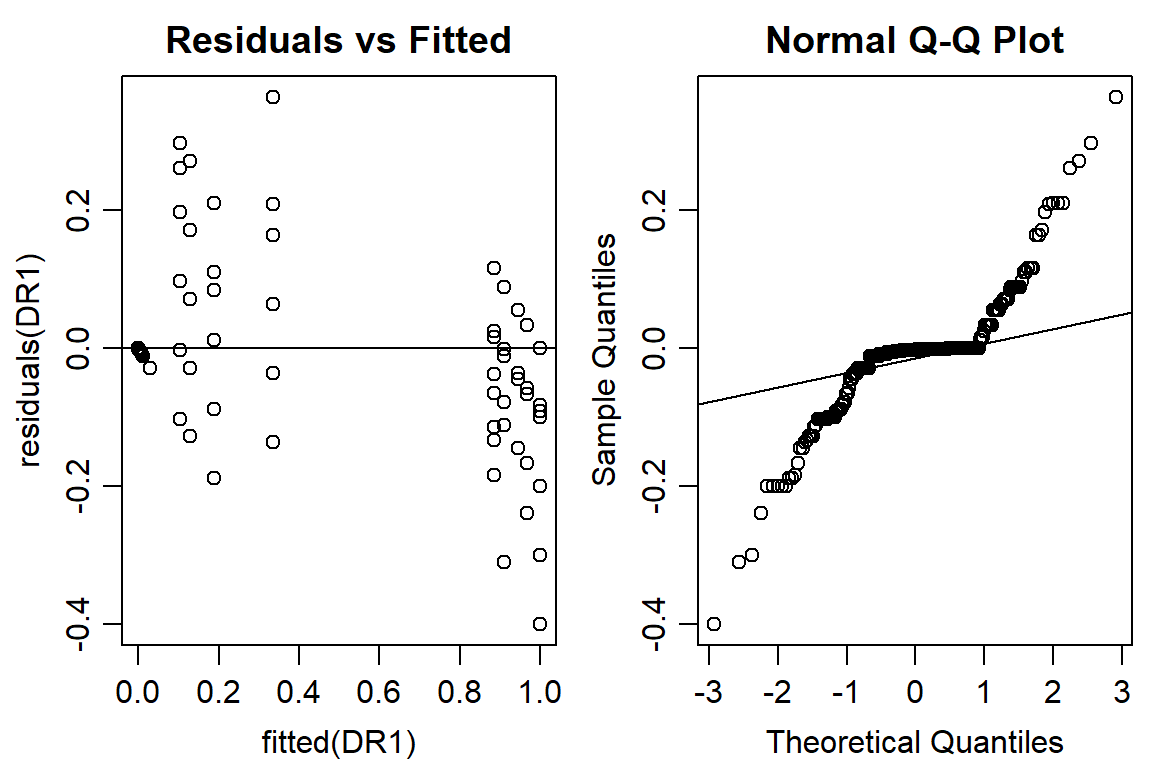
#shows slope of pupation, LD50 is significantly different than 0 for each instar
par(mfrow = c(1, 1), mar=c(3.2,3.2,.5,.5), mgp=c(2,.7,0))
plot(DR1, broken=TRUE, xlim=c(0,2), bty="l", xlab="Concentration", ylab="Survival to Pupation")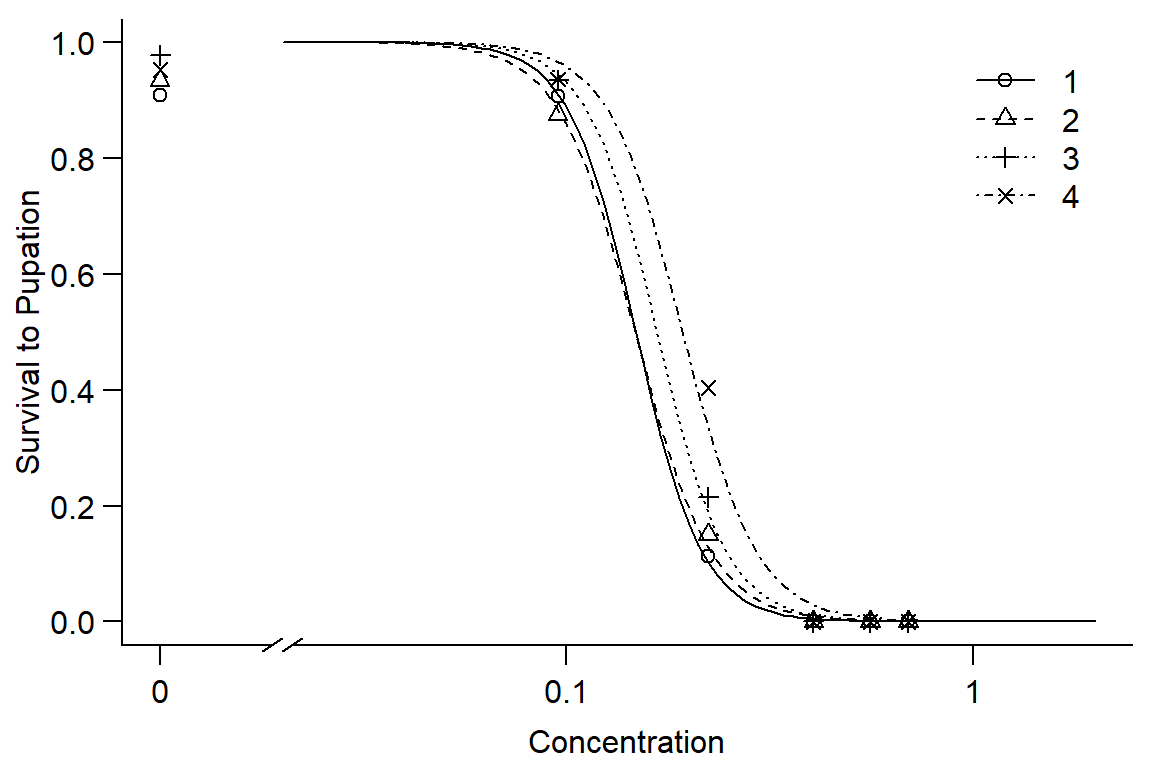
modelFit(DR1)## Goodness-of-fit test
##
## Df Chisq value p value
##
## DRC model 232 16.065 1EDcomp(DR1,c(50,50), reverse=TRUE)##
## Estimated ratios of effect doses
##
## Estimate Std. Error t-value p-value
## 2/1:50/50 0.997289 0.184569 -0.014688 0.988281
## 3/1:50/50 1.130243 0.205675 0.633247 0.526572
## 4/1:50/50 1.306015 0.230260 1.328998 0.183849
## 3/2:50/50 1.133315 0.207978 0.641007 0.521518
## 4/2:50/50 1.309565 0.232965 1.328803 0.183913
## 4/3:50/50 1.155517 0.201836 0.770511 0.440997#Instar has little effect on pupation, instars 1 and 2 very similar, 3 and 4 increasing survival. Overall, model doesn't fit well.Option 2: look at linear model
pairs(DR$`%Pupated` ~ (DR$Block) + (DR$Rep) + DR$Concentration + DR$Instar)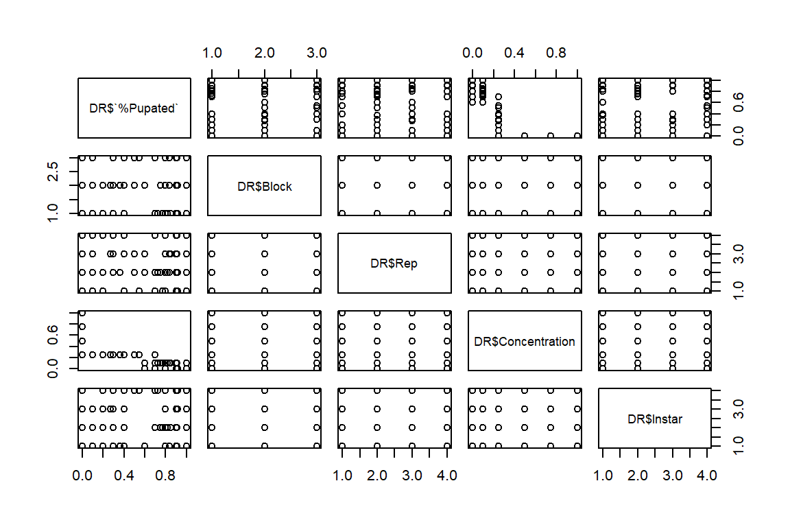
#Concentration has trend with % pupated; block/reps random, no pattern as expected. Instar appears to have little effect
op <- par(mfrow = c(1, 1), mar=c(3.2,3.2,0,.5), mgp=c(2,.7,0))
plot(DR$`%Pupated` ~ DR$Concentration, data = DR, bty="l")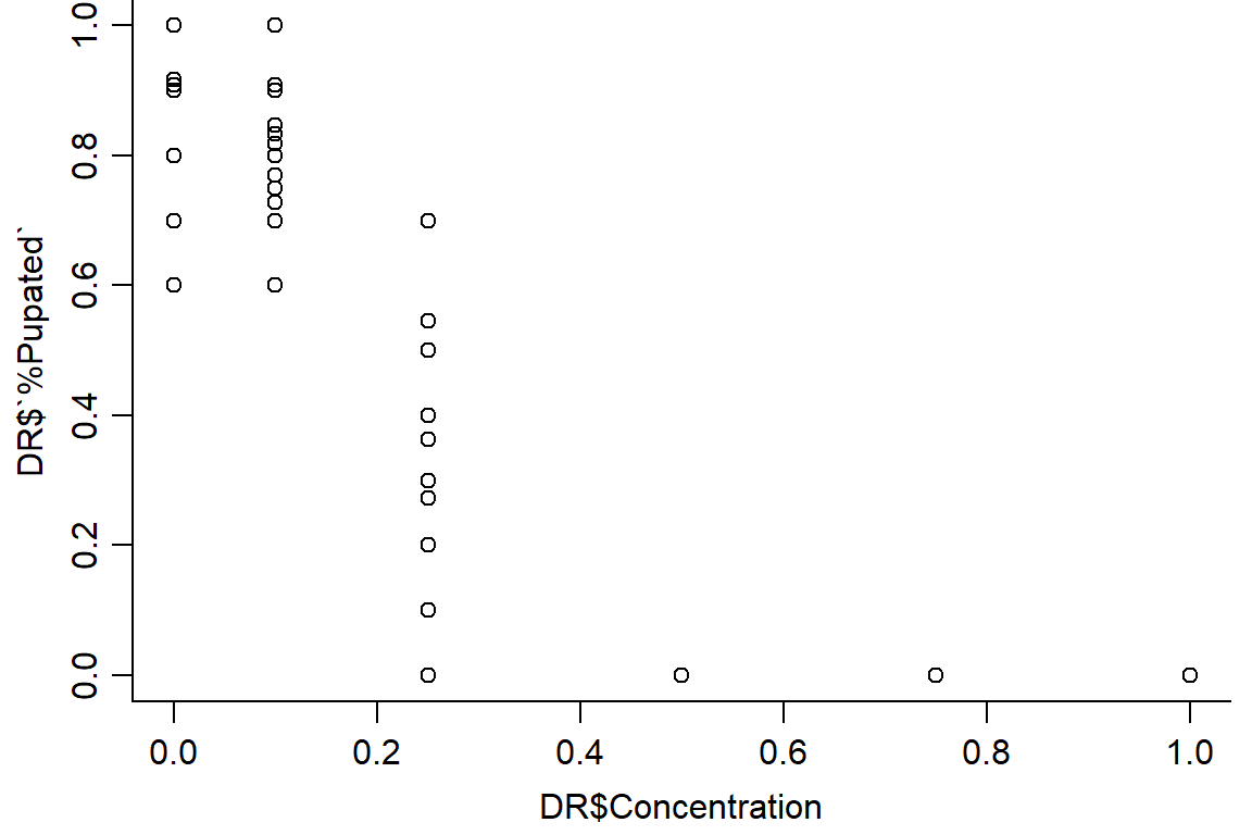
pupation.lm1 <- lm(DR$`%Pupated` ~ (Block) + (Rep) + Concentration + Instar + Concentration:Instar, data = DR)
summary(pupation.lm1)
##
## Call:
## lm(formula = DR$`%Pupated` ~ (Block) + (Rep) + Concentration +
## Instar + Concentration:Instar, data = DR)
##
## Residuals:
## Min 1Q Median 3Q Max
## -0.55033 -0.25374 -0.01523 0.21556 0.38197
##
## Coefficients:
## Estimate Std. Error t value Pr(>|t|)
## (Intercept) 0.667166 0.073091 9.128 <2e-16 ***
## Block 0.003084 0.017585 0.175 0.8609
## Rep 0.003364 0.012842 0.262 0.7936
## Concentration -0.895659 0.098928 -9.054 <2e-16 ***
## Instar 0.037893 0.020247 1.871 0.0623 .
## Concentration:Instar -0.039072 0.036123 -1.082 0.2803
## ---
## Signif. codes: 0 '***' 0.001 '**' 0.01 '*' 0.05 '.' 0.1 ' ' 1
##
## Residual standard error: 0.2437 on 282 degrees of freedom
## Multiple R-squared: 0.6835, Adjusted R-squared: 0.6778
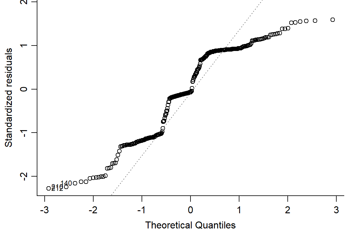
## F-statistic: 121.8 on 5 and 282 DF, p-value: < 2.2e-16plot(pupation.lm1, bty="l")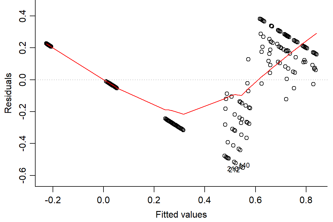
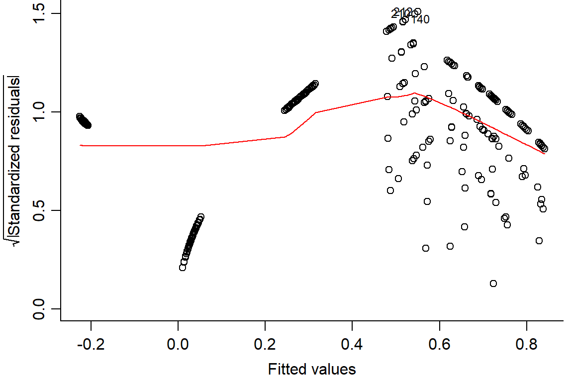
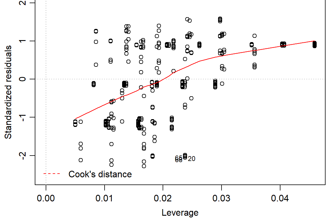
#look at residuals
op <- par(mfrow = c(1, 2), mar=c(3.2,3.2,2,.5), mgp=c(2,.7,0)) #put two graphs together
plot(residuals(pupation.lm1) ~ fitted(pupation.lm1), main="Residuals vs Fitted")
abline(h=0) #should look random
qqnorm(residuals(pupation.lm1))
qqline(residuals(pupation.lm1)) 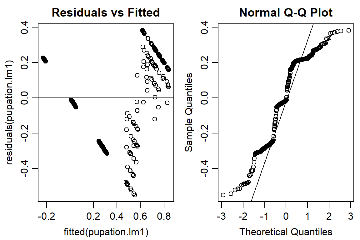
#not quite normal on QQ plot, residuals not random -> use logit or beta distribution#logit binomial dist
pupation.lm2 <- glm((DR$`%Pupated`)~ (DR$Block) + (DR$Rep) + (DR$Concentration) + (DR$Instar) + (DR$Concentration:DR$Instar), family = binomial(link = "logit"))
plot(pupation.lm2, bty="l")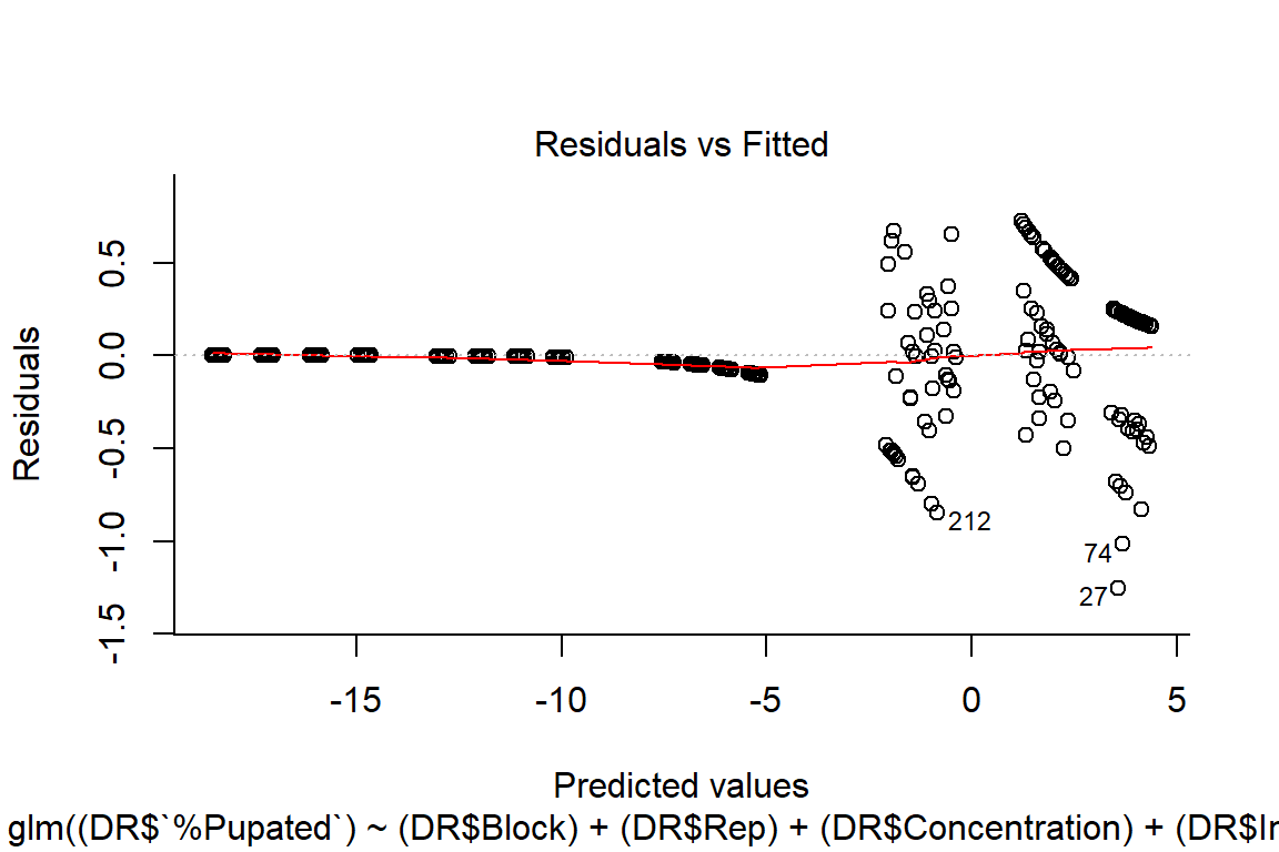
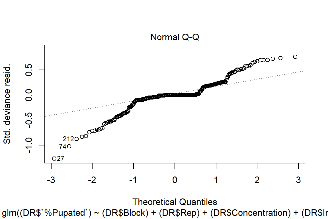
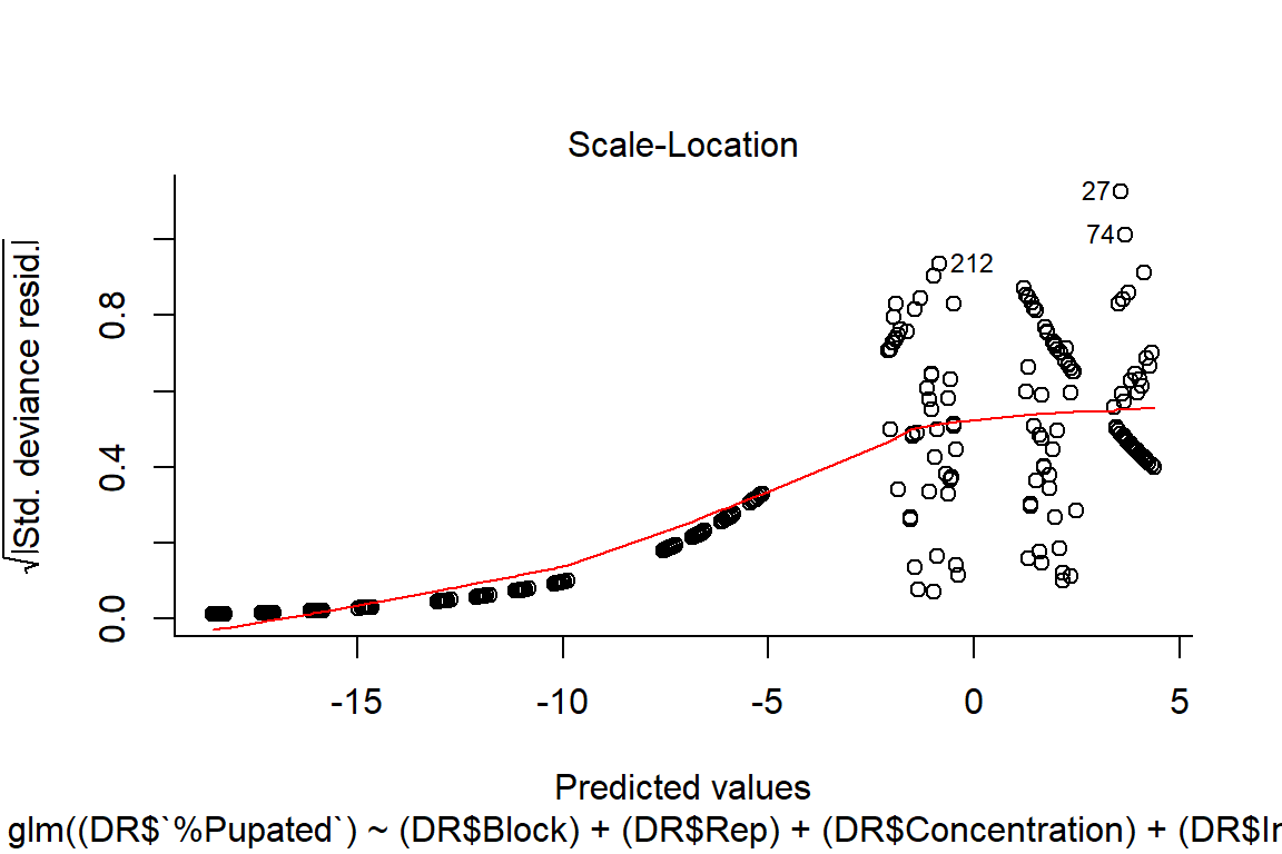
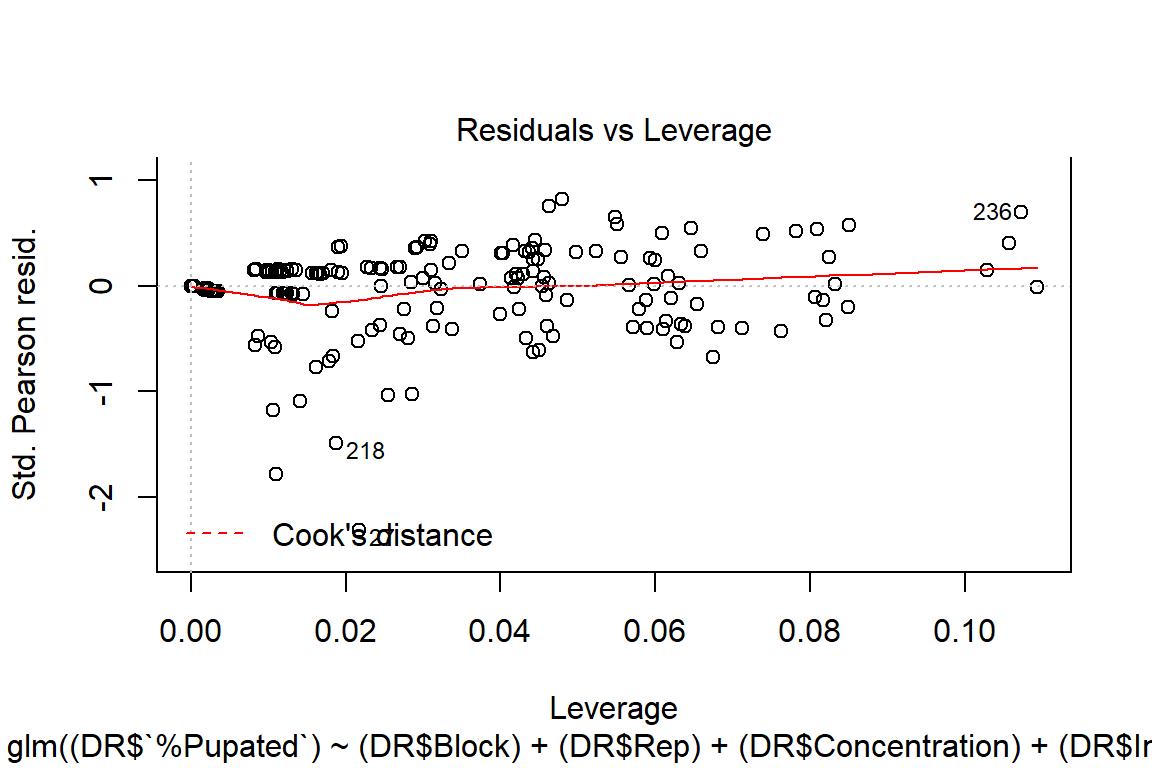
#look at residuals
plot(residuals(pupation.lm2) ~ fitted(pupation.lm2), main="Residuals vs Fitted")
abline(h=0) #should look random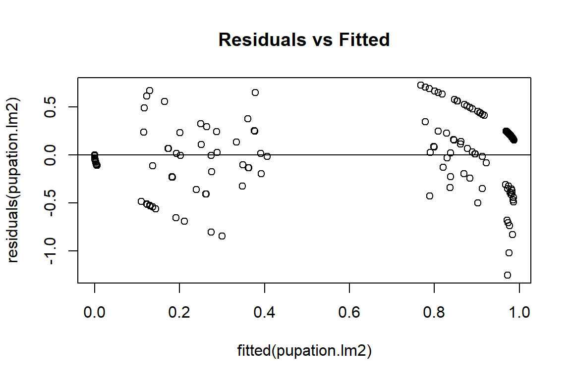
qqnorm(residuals(pupation.lm1))
qqline(residuals(pupation.lm1)) 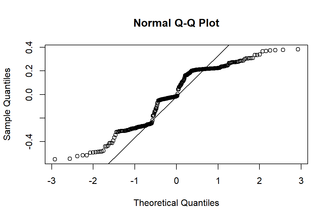
#residuals random, more normal on qqplot
summary(pupation.lm2)
##
## Call:
## glm(formula = (DR$`%Pupated`) ~ (DR$Block) + (DR$Rep) + (DR$Concentration) +
## (DR$Instar) + (DR$Concentration:DR$Instar), family = binomial(link = "logit"))
##
## Deviance Residuals:
## Min 1Q Median 3Q Max
## -1.25219 -0.06925 -0.00233 0.12168 0.72655
##
## Coefficients:
## Estimate Std. Error z value Pr(>|z|)
## (Intercept) 3.03900 1.56721 1.939 0.05249 .
## DR$Block 0.05845 0.31427 0.186 0.85247
## DR$Rep 0.06374 0.22962 0.278 0.78132
## DR$Concentration -22.86314 7.28283 -3.139 0.00169 **
## DR$Instar 0.22619 0.52014 0.435 0.66366
## DR$Concentration:DR$Instar 0.96115 2.62361 0.366 0.71411
## ---
## Signif. codes: 0 '***' 0.001 '**' 0.01 '*' 0.05 '.' 0.1 ' ' 1
##
## (Dispersion parameter for binomial family taken to be 1)
##
## Null deviance: 295.246 on 287 degrees of freedom
## Residual deviance: 24.113 on 282 degrees of freedom
## AIC: 58.259
##
## Number of Fisher Scoring iterations: 8#compare linear model with non linear, linear > DR2 due to much lower AIC
AIC(DR1, pupation.lm2)## df AIC
## DR1 8 245.08353
## pupation.lm2 6 58.25937Log-logistic and Weibull models
Other tools related to dose-response models
#compare log-logistic and Weibull models (pooling instar because non-significant)
DR0 <- drm(DR$`%Pupated` ~ DR$Concentration, data = DR, fct = LL.4())
DR1 <- drm(DR$`%Pupated` ~ DR$Concentration, data = DR, fct = W1.4())
DR2 <- drm(DR$`%Pupated` ~ DR$Concentration, data = DR, fct = W2.4())

par(mfrow=c(1,1), mar=c(3.2,3.2,.5,.5), mgp=c(2,.7,0))
plot(DR0, broken=TRUE, xlab="Conc", ylab="% Pupation", lwd=2, cex=1.2, cex.axis=1.2, cex.lab=1.2, bty="l")
plot(DR1, add=TRUE, broken=TRUE, lty=2, lwd=2) #Weibull-1
plot(DR2, add=TRUE, broken=TRUE, lty=3, lwd=2) #Weibull-2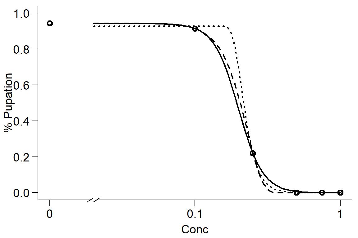
#Effective dose
ED(DR1,50,interval="delta")
##
## Estimated effective doses
##
## Estimate Std. Error Lower Upper
## e:1:50 0.2092415 0.0066148 0.1962212 0.2222618ED(DR1,90,interval="delta")##
## Estimated effective doses
##
## Estimate Std. Error Lower Upper
## e:1:90 0.2795042 0.0057066 0.2682715 0.2907369ED(DR1,95,interval="delta")##
## Estimated effective doses
##
## Estimate Std. Error Lower Upper
## e:1:95 0.2978175 0.0088051 0.2804860 0.3151490edLL<-data.frame(ED(DR0,c(10,50,90),interval="delta", display=FALSE),ll="Log-logistic")
edW1<-data.frame(ED(DR1,c(10,50,90),interval="delta", display=FALSE),ll="Weibull 1")
edW2<-data.frame(ED(DR2,c(10,50,90),interval="delta", display=FALSE),ll="Weibull 2")
CombED<-rbind(edLL,edW1,edW2)
p1 <- ggplot(data=CombED[c(1,4,7),], aes(x=ll, y=Estimate))+ geom_bar(stat="identity", fill="lightgreen", colour="black")+
geom_errorbar(aes(ymin=Lower, ymax=Upper), width=0.1) + ylab("ED10")+ xlab("")
p2 <- ggplot(data=CombED[c(2,5,8),], aes(x=ll, y=Estimate))+ geom_bar(stat="identity", fill="lightgreen", colour="black")+
geom_errorbar(aes(ymin=Lower, ymax=Upper), width=0.1) + ylab("ED50")+ xlab("")
p3 <- ggplot(data=CombED[c(3,6,9),], aes(x=ll, y=Estimate))+ geom_bar(stat="identity", fill="lightgreen", colour="black")+
geom_errorbar(aes(ymin=Lower, ymax=Upper), width=0.1) + ylab("ED90")+ xlab("Sigmoid four parameter models")
plot_grid(p1,p2,p3, ncol=1)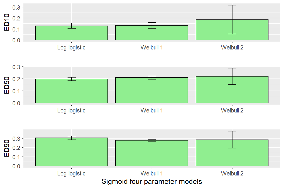
#look at different tests, either Log-logistic or Weibull 1 most appropriate

comped(CombED[c(1,4),1],CombED[c(1,4),2],log=F,operator = "-")
##
## Estimated difference of effective doses
##
## Estimate Std. Error Lower Upper
## [1,] -0.0034982 0.0186068 -0.0399669 0.033Mortality Example 24 hr
Look at Day 1 (24hr Mortality)
summary(DR)## Concentration Instar Block Rep Total Pupae %Pupated Day0 Day1p Day2p Day3p Day4p Day5p Day6p Day7p Day8p Day9p Day10p Day11p Day12p Day13p Day14p
## Min. :0.0000 Min. :1.00 Min. :1 Min. :1.00 Min. :10.00 Min. : 0.000 Min. :0.000 Min. :10.00 Min. :0.0000 Min. :0.0000 Min. :0.0000 Min. :0.00000 Min. :0.0000 Min. :0.0000 Min. :0.0000 Min. :0.0000 Min. :0.0000 Min. :0.0000 Min. :0.0000 Min. :0.0000 Min. :0.0000 Min. :0.0000
## 1st Qu.:0.1000 1st Qu.:1.75 1st Qu.:1 1st Qu.:1.75 1st Qu.:10.00 1st Qu.: 0.000 1st Qu.:0.000 1st Qu.:10.00 1st Qu.:0.0000 1st Qu.:0.0000 1st Qu.:0.0000 1st Qu.:0.08333 1st Qu.:0.1000 1st Qu.:0.1000 1st Qu.:0.1000 1st Qu.:0.1000 1st Qu.:0.1000 1st Qu.:0.1000 1st Qu.:0.1404 1st Qu.:0.1404 1st Qu.:0.4000 1st Qu.:0.4000
## Median :0.3750 Median :2.50 Median :2 Median :2.50 Median :10.00 Median : 0.000 Median :0.000 Median :10.00 Median :0.3000 Median :0.6500 Median :0.7500 Median :0.80000 Median :0.8500 Median :0.9000 Median :0.9000 Median :1.0000 Median :1.0000 Median :1.0000 Median :1.0000 Median :1.0000 Median :1.0000 Median :1.0000
## Mean :0.4333 Mean :2.50 Mean :2 Mean :2.50 Mean :10.17 Mean : 3.615 Mean :0.346 Mean :10.17 Mean :0.3924 Mean :0.5186 Mean :0.5499 Mean :0.56945 Mean :0.5846 Mean :0.6026 Mean :0.6179 Mean :0.6258 Mean :0.6367 Mean :0.6425 Mean :0.6745 Mean :0.6778 Mean :0.7434 Mean :0.7454
## 3rd Qu.:0.7500 3rd Qu.:3.25 3rd Qu.:3 3rd Qu.:3.25 3rd Qu.:10.00 3rd Qu.: 9.000 3rd Qu.:0.900 3rd Qu.:10.00 3rd Qu.:0.8000 3rd Qu.:1.0000 3rd Qu.:1.0000 3rd Qu.:1.00000 3rd Qu.:1.0000 3rd Qu.:1.0000 3rd Qu.:1.0000 3rd Qu.:1.0000 3rd Qu.:1.0000 3rd Qu.:1.0000 3rd Qu.:1.0000 3rd Qu.:1.0000 3rd Qu.:1.0000 3rd Qu.:1.0000
## Max. :1.0000 Max. :4.00 Max. :3 Max. :4.00 Max. :14.00 Max. :14.000 Max. :1.000 Max. :14.00 Max. :1.0000 Max. :1.0000 Max. :1.0000 Max. :1.00000 Max. :1.0000 Max. :1.0000 Max. :1.0000 Max. :1.0000 Max. :1.0000 Max. :1.0000 Max. :1.0000 Max. :1.0000 Max. :1.0000 Max. :1.0000op <- par(mfrow = c(1, 2), mar=c(3.2,3.2,2,.5), mgp=c(2,.7,0))
plot(DR$Day1p~ DR$Concentration, data = DR, main="Original Dose Scale")
plot(DR$Day1p ~ logit(DR$Concentration+0.01), data = DR, main="Logarithmic Dose Scale")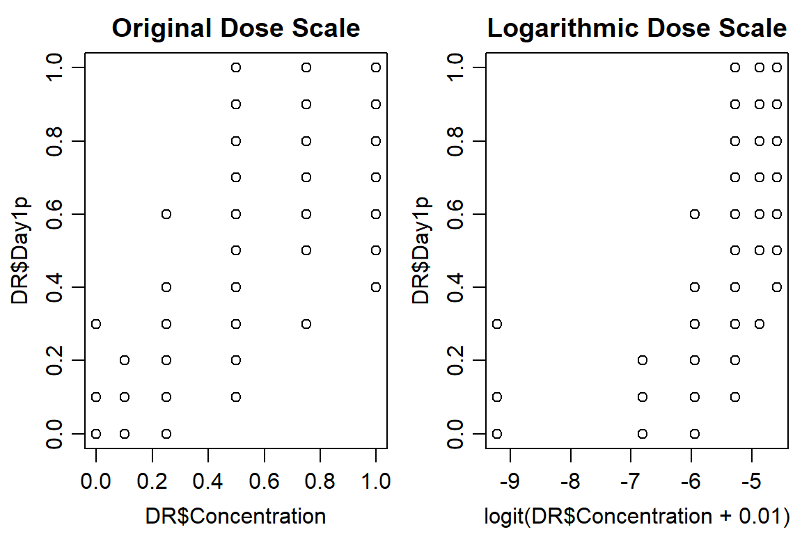
#Look at control data, make sure mortality is < ~ 5%
aggregate(DR[,9], list(DR$Concentration), mean)
## Group.1 Day1p
## 1 0.00 0.02083333
## 2 0.10 0.01666667
## 3 0.25 0.09166667
## 4 0.50 0.55416667
## 5 0.75 0.78541667
## 6 1.00 0.88541667Option 1:
#option 1: use DR
Day1DR<-drm(DR$Day1p ~ DR$Concentration, DR$Instar, data = DR, fct=LL.2(names=c("Slope", "LD50")), type=("binomial"), na.action=na.omit)
summary(Day1DR)
##
## Model fitted: Log-logistic (ED50 as parameter) with lower limit at 0 and upper limit at 1 (2 parms)
##
## Parameter estimates:
##
## Estimate Std. Error t-value p-value
## Slope:1 -2.384882 0.608538 -3.9190 8.890e-05 ***
## Slope:2 -3.182438 0.801062 -3.9728 7.104e-05 ***
## Slope:3 -3.345483 0.905529 -3.6945 0.0002203 ***
## Slope:4 -3.460856 0.880632 -3.9300 8.496e-05 ***
## LD50:1 0.457671 0.066102 6.9237 4.400e-12 ***
## LD50:2 0.461353 0.056611 8.1495 4.047e-16 ***
## LD50:3 0.561857 0.062752 8.9536 < 2.2e-16 ***
## LD50:4 0.470069 0.054920 8.5592 < 2.2e-16 ***
## ---
## Signif. codes: 0 '***' 0.001 '**' 0.01 '*' 0.05 '.' 0.1 ' ' 1#shows slope, LD50 is significantly different than 0 for each instar
par(mfrow = c(1, 1), mar=c(3.2,3.2,.5,.5), mgp=c(2,.7,0))
plot(Day1DR, broken=TRUE, xlim=c(0,2), bty="l", xlab="Concentration", ylab="Mortality")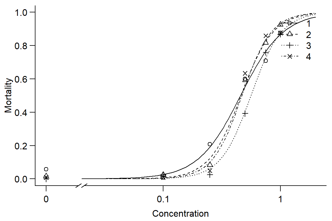
EDcomp(Day1DR,c(50,50), reverse=TRUE)##
## Estimated ratios of effect doses
##
## Estimate Std. Error t-value p-value
## 2/1:50/50 1.008045 0.191044 0.042111 0.966410
## 3/1:50/50 1.227643 0.224140 1.015629 0.309806
## 4/1:50/50 1.027089 0.190803 0.141975 0.887100
## 3/2:50/50 1.217845 0.202070 1.078068 0.281003
## 4/2:50/50 1.018892 0.172632 0.109437 0.912856
## 4/3:50/50 0.836635 0.135225 -1.208096 0.227010#Instar has little effect on mortality, instars 1 and 2 similar, 3 and 4 less responsive. Overall, model doesn't fit well.
#look at residuals
op <- par(mfrow = c(1, 2), mar=c(3.2,3.2,2,.5), mgp=c(2,.7,0))
plot(residuals(Day1DR) ~ fitted(Day1DR), main="Residuals vs Fitted")
qqnorm(residuals(Day1DR))
qqline(residuals(Day1DR)) 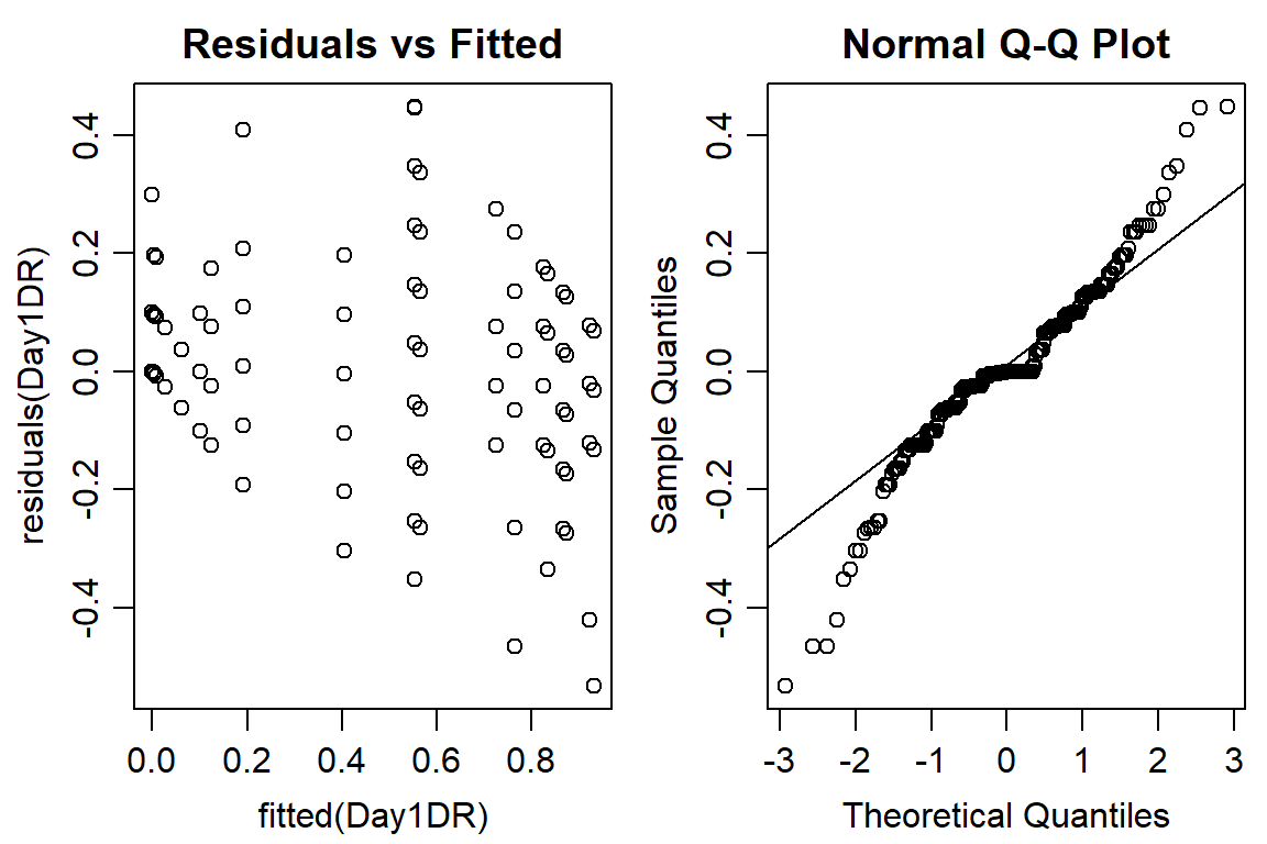
#data not normally distributed

op <- par(mfrow = c(1, 2), mar=c(3.2,3.2,.5,.5), mgp=c(2,.7,0))
plot(Day1DR, broken=TRUE, bty="l", xlab="Conc", ylab="Mortality")
plot(Day1DR, broken=TRUE, bty="l", xlab="Concentration", ylab="Mortality",type="all")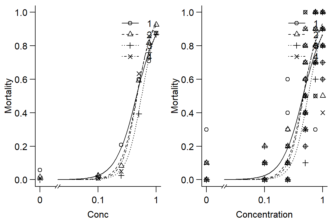
modelFit(Day1DR)## Goodness-of-fit test
##
## Df Chisq value p value
##
## DRC model 232 57.143 1#model doesn't fit very well, instar doesnt have much effect on DROption 2:
#Option 2: look at linear model
pairs(DR$Day1p ~ (DR$Block) + (DR$Rep) + DR$Concentration + DR$Instar)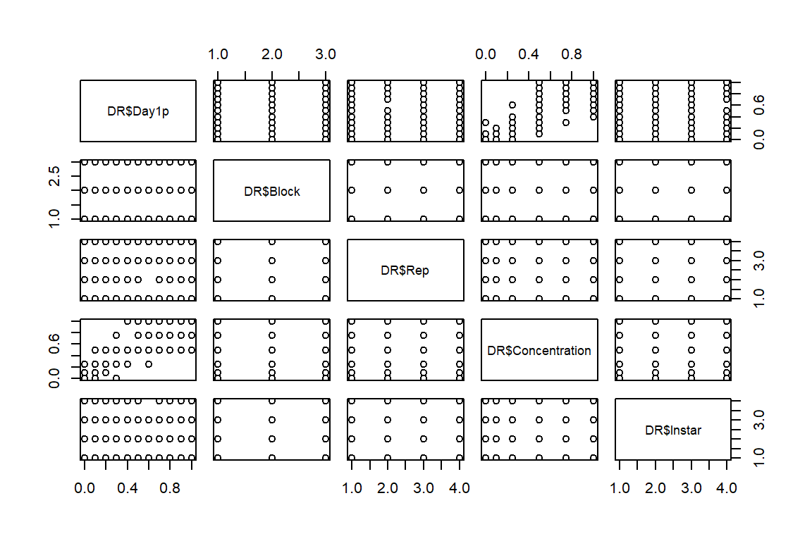
op <- par(mfrow = c(1, 1), mar=c(3.2,3.2,0,.5), mgp=c(2,.7,0))
plot(DR$Day1p ~ DR$Concentration, data = DR, bty="l")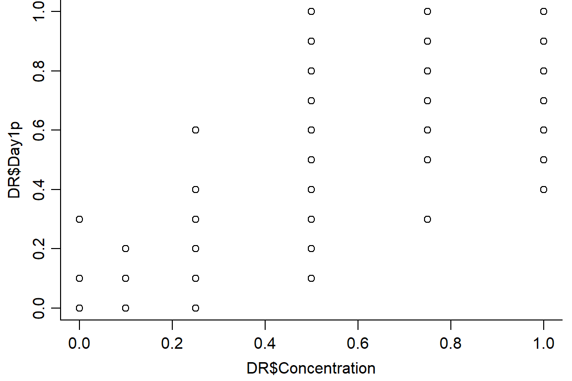
day1.lm <- lm(DR$Day1p ~ (Block) + (Rep) + Concentration + Instar + Concentration:Instar, data = DR)
summary(day1.lm)
##
## Call:
## lm(formula = DR$Day1p ~ (Block) + (Rep) + Concentration + Instar +
## Concentration:Instar, data = DR)
##
## Residuals:
## Min 1Q Median 3Q Max
## -0.56986 -0.08445 0.00331 0.07096 0.53949
##
## Coefficients:
## Estimate Std. Error t value Pr(>|t|)
## (Intercept) 0.021339 0.048693 0.438 0.6615
## Block 0.005729 0.011715 0.489 0.6252
## Rep -0.006667 0.008556 -0.779 0.4365
## Concentration 0.913095 0.065906 13.855 <2e-16 ***
## Instar -0.022310 0.013489 -1.654 0.0993 .
## Concentration:Instar 0.033535 0.024065 1.393 0.1646
## ---
## Signif. codes: 0 '***' 0.001 '**' 0.01 '*' 0.05 '.' 0.1 ' ' 1
##
## Residual standard error: 0.1623 on 282 degrees of freedom
## Multiple R-squared: 0.83, Adjusted R-squared: 0.827
## F-statistic: 275.3 on 5 and 282 DF, p-value: < 2.2e-16plot(day1.lm, which=1, bty="l")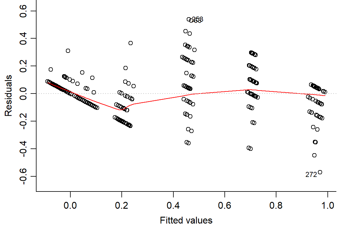
#look at residuals
plot(residuals(day1.lm) ~ fitted(day1.lm), main="Residuals vs Fitted")
abline(h=0) #should look random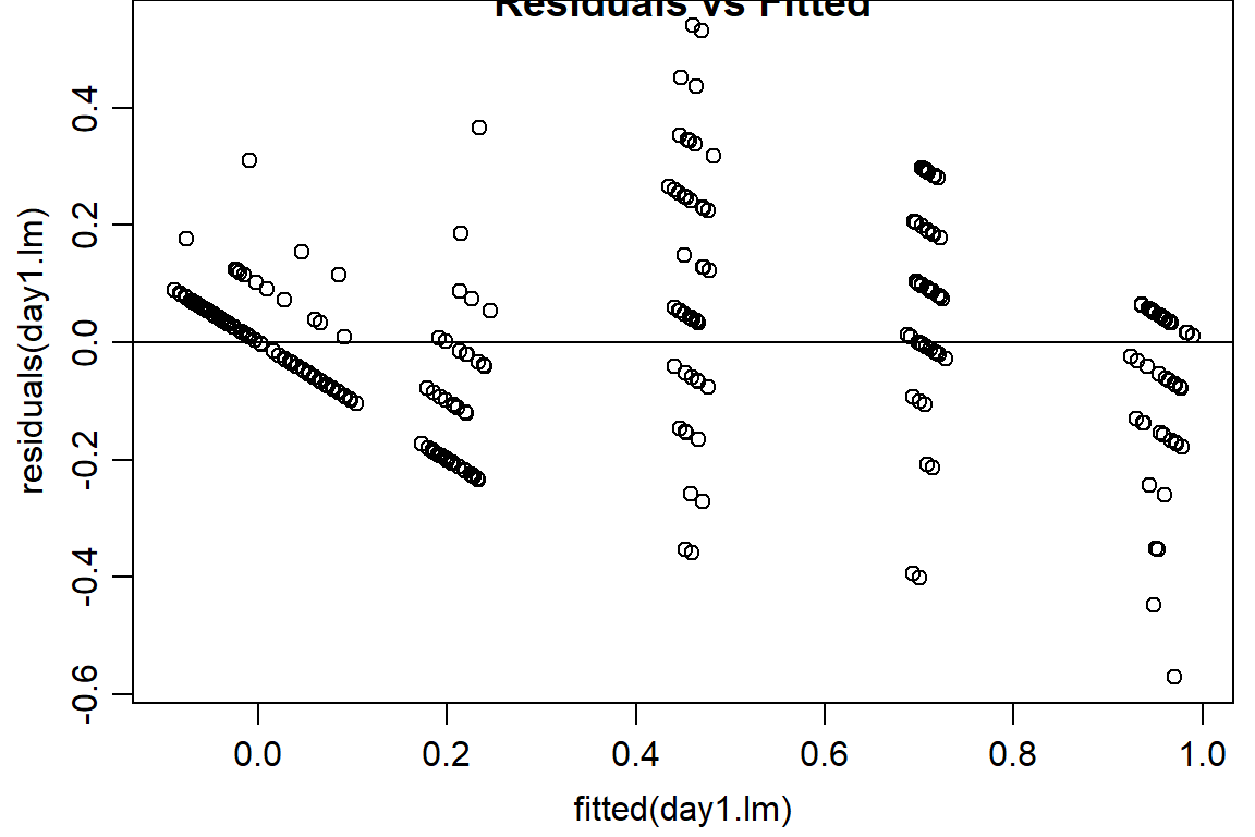
qqnorm(residuals(day1.lm))
qqline(residuals(day1.lm)) 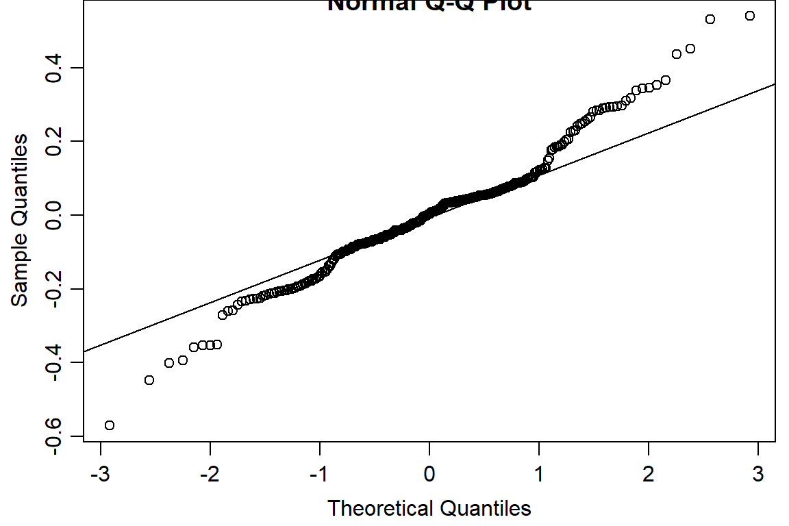
# fit with binomial dist
day1.lm2 <- glm((DR$Day1p)~ (DR$Block) + (DR$Rep) + (DR$Concentration) + (DR$Instar) + (DR$Concentration:DR$Instar), family = binomial(link = "logit"))
## Warning in eval(family$initialize): non-integer #successes in a binomial glm!summary(day1.lm2)##
## Call:
## glm(formula = (DR$Day1p) ~ (DR$Block) + (DR$Rep) + (DR$Concentration) +
## (DR$Instar) + (DR$Concentration:DR$Instar), family = binomial(link = "logit"))
##
## Deviance Residuals:
## Min 1Q Median 3Q Max
## -1.6080 -0.3367 -0.1780 0.2638 1.3359
##
## Coefficients:
## Estimate Std. Error z value Pr(>|z|)
## (Intercept) -2.51902 1.05333 -2.391 0.01678 *
## DR$Block 0.05248 0.21850 0.240 0.81017
## DR$Rep -0.06107 0.15964 -0.383 0.70205
## DR$Concentration 4.84531 1.53331 3.160 0.00158 **
## DR$Instar -0.39914 0.35381 -1.128 0.25926
## DR$Concentration:DR$Instar 0.64192 0.61519 1.043 0.29674
## ---
## Signif. codes: 0 '***' 0.001 '**' 0.01 '*' 0.05 '.' 0.1 ' ' 1
##
## (Dispersion parameter for binomial family taken to be 1)
##
## Null deviance: 234.383 on 287 degrees of freedom
## Residual deviance: 53.056 on 282 degrees of freedom
## AIC: 153.42
##
## Number of Fisher Scoring iterations: 6plot(day1.lm2, which=1, bty="l")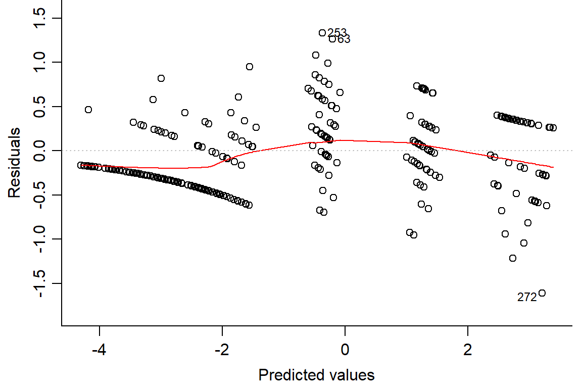
plot(residuals(day1.lm2) ~ fitted(day1.lm2), main="Residuals vs Fitted")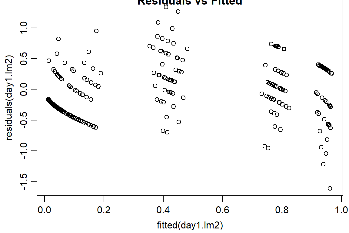
qqnorm(residuals(day1.lm2))
qqline(residuals(day1.lm2)) 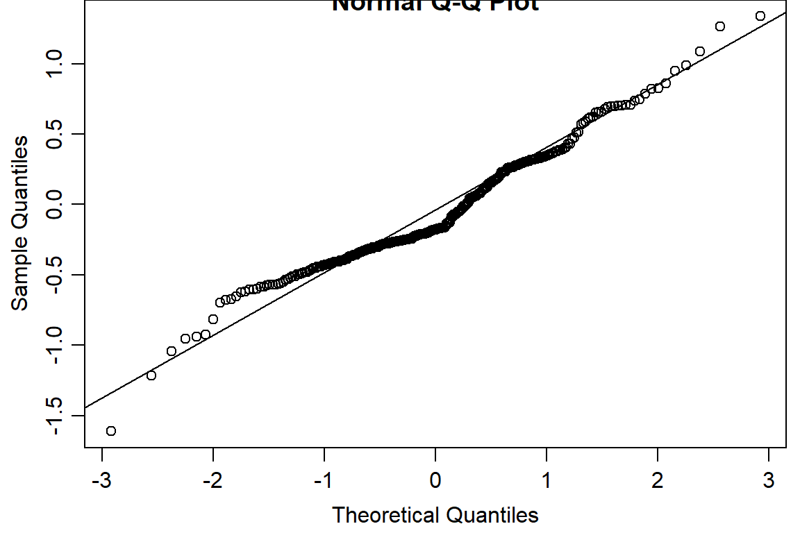
#binomial logit fits better#compare linear model with DR, linear > DR due to lower AIC
AIC(Day1DR, day1.lm2, k=2)## df AIC
## Day1DR 8 256.6130
## day1.lm2 6 153.4244summary(day1.lm2)##
## Call:
## glm(formula = (DR$Day1p) ~ (DR$Block) + (DR$Rep) + (DR$Concentration) +
## (DR$Instar) + (DR$Concentration:DR$Instar), family = binomial(link = "logit"))
##
## Deviance Residuals:
## Min 1Q Median 3Q Max
## -1.6080 -0.3367 -0.1780 0.2638 1.3359
##
## Coefficients:
## Estimate Std. Error z value Pr(>|z|)
## (Intercept) -2.51902 1.05333 -2.391 0.01678 *
## DR$Block 0.05248 0.21850 0.240 0.81017
## DR$Rep -0.06107 0.15964 -0.383 0.70205
## DR$Concentration 4.84531 1.53331 3.160 0.00158 **
## DR$Instar -0.39914 0.35381 -1.128 0.25926
## DR$Concentration:DR$Instar 0.64192 0.61519 1.043 0.29674
## ---
## Signif. codes: 0 '***' 0.001 '**' 0.01 '*' 0.05 '.' 0.1 ' ' 1
##
## (Dispersion parameter for binomial family taken to be 1)
##
## Null deviance: 234.383 on 287 degrees of freedom
## Residual deviance: 53.056 on 282 degrees of freedom
## AIC: 153.42
##
## Number of Fisher Scoring iterations: 6Other Tools:
#Using drm package to determine effective dose.
#compare log-logistic and Weibull models (pooling instar because non-significant)
Day1DR <- drm(DR$Day1p ~ DR$Concentration, data = DR, fct = LL.4())
Day1DR2 <- drm(DR$Day1p ~ DR$Concentration, data = DR, fct = W1.4())
Day1DR3 <- drm(DR$Day1p ~ DR$Concentration, data = DR, fct = W2.4())

par(mfrow=c(1,1), mar=c(3.2,3.2,.5,.5), mgp=c(2,.7,0))
plot(Day1DR, broken=TRUE, xlab="Conc", ylab="% Pupation", lwd=2, cex=1.2, cex.axis=1.2, cex.lab=1.2, bty="l")
plot(Day1DR2, add=TRUE, broken=TRUE, lty=2, lwd=2) #Weibull-1
plot(Day1DR3, add=TRUE, broken=TRUE, lty=3, lwd=2) #Weibull-2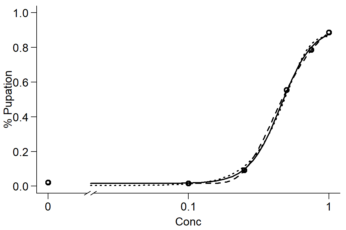
#Effective dose using log-logistic model
ED(Day1DR,50,interval="delta")
##
## Estimated effective doses
##
## Estimate Std. Error Lower Upper
## e:1:50 0.45532 0.01532 0.42517 0.48548ED(Day1DR,90,interval="delta")##
## Estimated effective doses
##
## Estimate Std. Error Lower Upper
## e:1:90 0.809377 0.069525 0.672527 0.946227ED(Day1DR,95,interval="delta")##
## Estimated effective doses
##
## Estimate Std. Error Lower Upper
## e:1:95 0.98426 0.10692 0.77380 1.19473edLL<-data.frame(ED(Day1DR,c(10,50,90),interval="delta", display=FALSE),ll="Log-logistic")
edW1<-data.frame(ED(Day1DR2,c(10,50,90),interval="delta", display=FALSE),ll="Weibull 1")
edW2<-data.frame(ED(Day1DR3,c(10,50,90),interval="delta", display=FALSE),ll="Weibull 2")
CombED<-rbind(edLL,edW1,edW2)
p1 <- ggplot(data=CombED[c(1,4,7),], aes(x=ll, y=Estimate))+ geom_bar(stat="identity", fill="lightgreen", colour="black")+
geom_errorbar(aes(ymin=Lower, ymax=Upper), width=0.1) + ylab("ED10")+ xlab("")
p2 <- ggplot(data=CombED[c(2,5,8),], aes(x=ll, y=Estimate))+ geom_bar(stat="identity", fill="lightgreen", colour="black")+
geom_errorbar(aes(ymin=Lower, ymax=Upper), width=0.1) + ylab("ED50")+ xlab("")
p3 <- ggplot(data=CombED[c(3,6,9),], aes(x=ll, y=Estimate))+ geom_bar(stat="identity", fill="lightgreen", colour="black")+
geom_errorbar(aes(ymin=Lower, ymax=Upper), width=0.1) + ylab("ED90")+ xlab("Sigmoid four parameter models")
plot_grid(p1,p2,p3, ncol=1)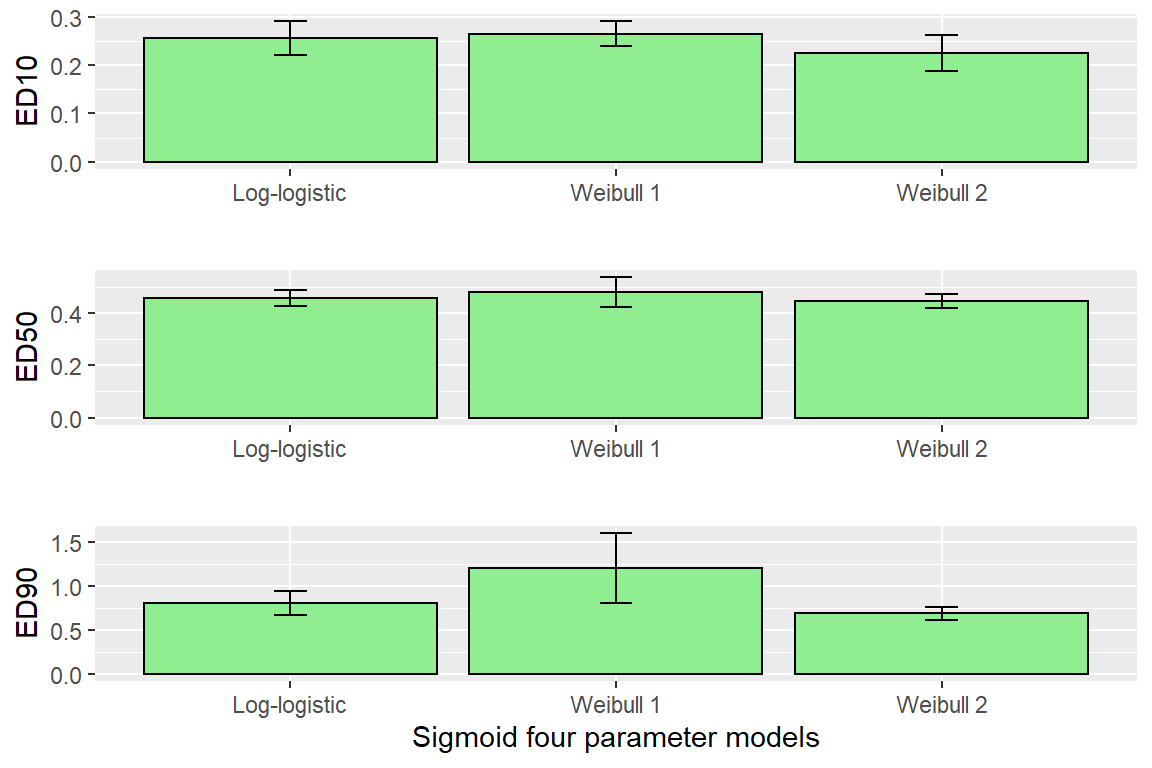
Mortality Example 48 hr
Look at Day 2 (48hr) Mortality
summary(DR)## Concentration Instar Block Rep Total Pupae %Pupated Day0 Day1p Day2p Day3p Day4p Day5p Day6p Day7p Day8p Day9p Day10p Day11p Day12p Day13p Day14p
## Min. :0.0000 Min. :1.00 Min. :1 Min. :1.00 Min. :10.00 Min. : 0.000 Min. :0.000 Min. :10.00 Min. :0.0000 Min. :0.0000 Min. :0.0000 Min. :0.00000 Min. :0.0000 Min. :0.0000 Min. :0.0000 Min. :0.0000 Min. :0.0000 Min. :0.0000 Min. :0.0000 Min. :0.0000 Min. :0.0000 Min. :0.0000
## 1st Qu.:0.1000 1st Qu.:1.75 1st Qu.:1 1st Qu.:1.75 1st Qu.:10.00 1st Qu.: 0.000 1st Qu.:0.000 1st Qu.:10.00 1st Qu.:0.0000 1st Qu.:0.0000 1st Qu.:0.0000 1st Qu.:0.08333 1st Qu.:0.1000 1st Qu.:0.1000 1st Qu.:0.1000 1st Qu.:0.1000 1st Qu.:0.1000 1st Qu.:0.1000 1st Qu.:0.1404 1st Qu.:0.1404 1st Qu.:0.4000 1st Qu.:0.4000
## Median :0.3750 Median :2.50 Median :2 Median :2.50 Median :10.00 Median : 0.000 Median :0.000 Median :10.00 Median :0.3000 Median :0.6500 Median :0.7500 Median :0.80000 Median :0.8500 Median :0.9000 Median :0.9000 Median :1.0000 Median :1.0000 Median :1.0000 Median :1.0000 Median :1.0000 Median :1.0000 Median :1.0000
## Mean :0.4333 Mean :2.50 Mean :2 Mean :2.50 Mean :10.17 Mean : 3.615 Mean :0.346 Mean :10.17 Mean :0.3924 Mean :0.5186 Mean :0.5499 Mean :0.56945 Mean :0.5846 Mean :0.6026 Mean :0.6179 Mean :0.6258 Mean :0.6367 Mean :0.6425 Mean :0.6745 Mean :0.6778 Mean :0.7434 Mean :0.7454
## 3rd Qu.:0.7500 3rd Qu.:3.25 3rd Qu.:3 3rd Qu.:3.25 3rd Qu.:10.00 3rd Qu.: 9.000 3rd Qu.:0.900 3rd Qu.:10.00 3rd Qu.:0.8000 3rd Qu.:1.0000 3rd Qu.:1.0000 3rd Qu.:1.00000 3rd Qu.:1.0000 3rd Qu.:1.0000 3rd Qu.:1.0000 3rd Qu.:1.0000 3rd Qu.:1.0000 3rd Qu.:1.0000 3rd Qu.:1.0000 3rd Qu.:1.0000 3rd Qu.:1.0000 3rd Qu.:1.0000
## Max. :1.0000 Max. :4.00 Max. :3 Max. :4.00 Max. :14.00 Max. :14.000 Max. :1.000 Max. :14.00 Max. :1.0000 Max. :1.0000 Max. :1.0000 Max. :1.00000 Max. :1.0000 Max. :1.0000 Max. :1.0000 Max. :1.0000 Max. :1.0000 Max. :1.0000 Max. :1.0000 Max. :1.0000 Max. :1.0000 Max. :1.0000op <- par(mfrow = c(1, 2), mar=c(3.2,3.2,2,.5), mgp=c(2,.7,0))
plot(DR$Day2p ~ DR$Concentration, data = DR, main="Original Dose Scale")
plot(DR$Day2p ~ logit(DR$Concentration+0.01), data = DR, main="Logarithmic Dose Scale")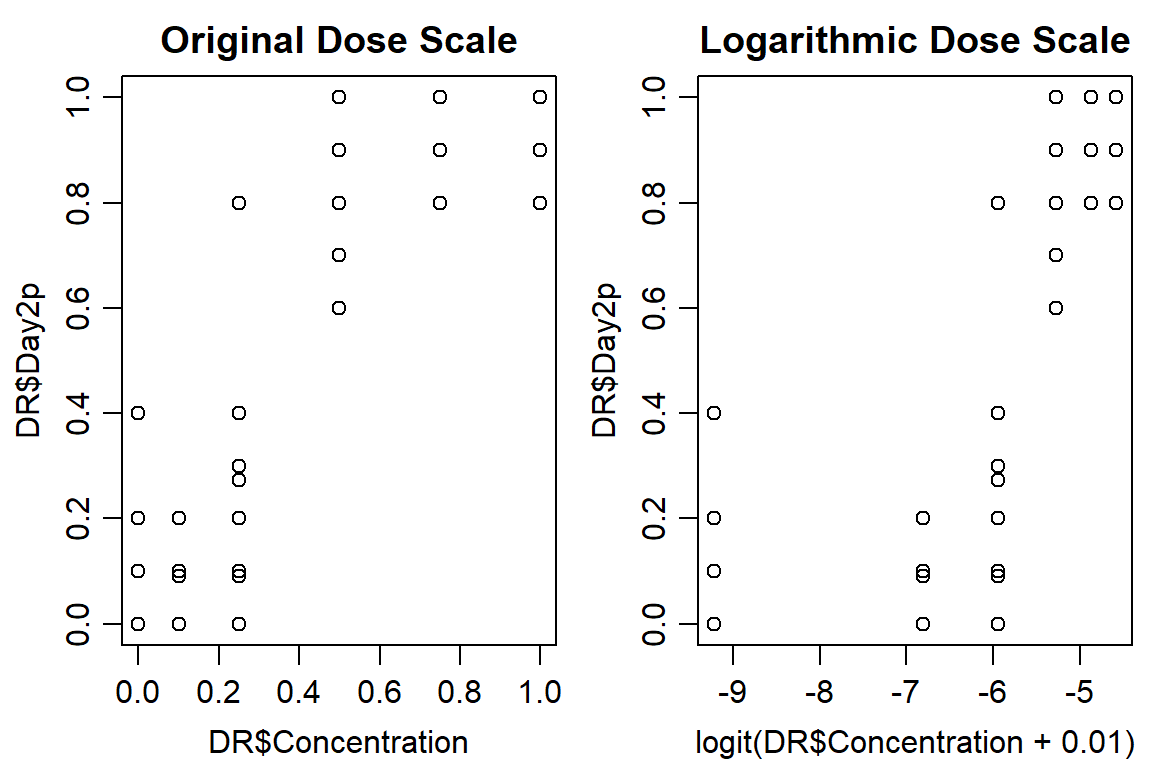
#Look at control data, make sure mortality is < ~ 5%
aggregate(DR[,10], list(DR$Concentration), mean)
## Group.1 Day2p
## 1 0.00 0.02500000
## 2 0.10 0.02689394
## 3 0.25 0.18882576
## 4 0.50 0.90416667
## 5 0.75 0.98541667
## 6 1.00 0.98125000Option 1: Dose Response Curve
#option 1: use DR
Day2DR<-drm(DR$Day2p ~ (DR$Concentration), DR$Instar, data = DR, fct=LL.2(names=c("Slope", "LD50")), type=("binomial"), na.action=na.omit)
summary(Day2DR)
##
## Model fitted: Log-logistic (ED50 as parameter) with lower limit at 0 and upper limit at 1 (2 parms)
##
## Parameter estimates:
##
## Estimate Std. Error t-value p-value
## Slope:1 -4.275095 1.136144 -3.7628 0.0001680 ***
## Slope:2 -3.852419 0.963761 -3.9973 6.408e-05 ***
## Slope:3 -5.163489 1.361471 -3.7926 0.0001491 ***
## Slope:4 -4.556448 1.151696 -3.9563 7.612e-05 ***
## LD50:1 0.299385 0.035025 8.5478 < 2.2e-16 ***
## LD50:2 0.317748 0.039065 8.1339 4.299e-16 ***
## LD50:3 0.333927 0.036185 9.2284 < 2.2e-16 ***
## LD50:4 0.347131 0.039313 8.8299 < 2.2e-16 ***
## ---
## Signif. codes: 0 '***' 0.001 '**' 0.01 '*' 0.05 '.' 0.1 ' ' 1#shows slope, LD50 is significantly different than 0 for each instar
par(mfrow = c(1, 1), mar=c(3.2,3.2,.5,.5), mgp=c(2,.7,0))
plot(Day2DR, broken=TRUE, xlim=c(0,2), bty="l", xlab="Concentration", ylab="Mortality")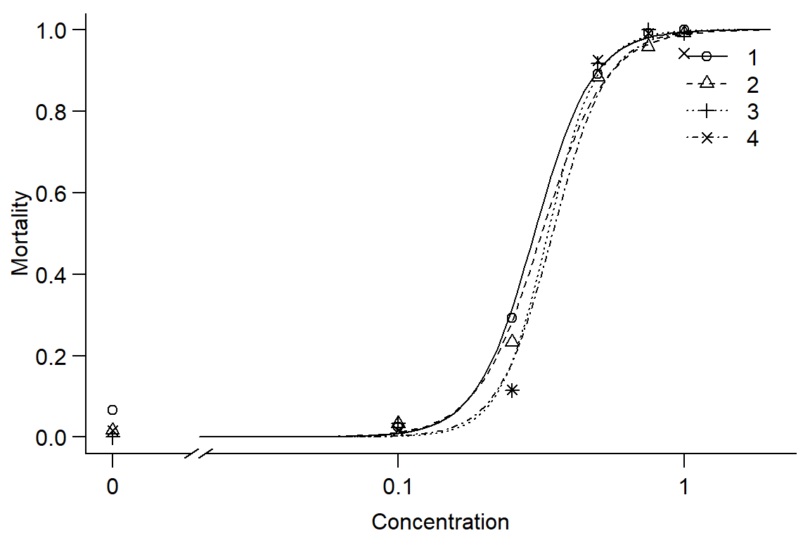
EDcomp(Day2DR,c(50,50), reverse=TRUE)##
## Estimated ratios of effect doses
##
## Estimate Std. Error t-value p-value
## 2/1:50/50 1.06134 0.18012 0.34053 0.73345
## 3/1:50/50 1.11538 0.17786 0.64870 0.51653
## 4/1:50/50 1.15948 0.18879 0.84473 0.39826
## 3/2:50/50 1.05092 0.17223 0.29566 0.76749
## 4/2:50/50 1.09247 0.18261 0.50639 0.61259
## 4/3:50/50 1.03954 0.16294 0.24266 0.80827#Instar has little effect on mortality, instars 1 and 2 similar, 3 and 4 less responsive. Overall, model doesn't fit well.
#look at residuals
op <- par(mfrow = c(1, 2), mar=c(3.2,3.2,2,.5), mgp=c(2,.7,0))
plot(residuals(Day2DR) ~ fitted(Day2DR), main="Residuals vs Fitted")
qqnorm(residuals(Day2DR))
qqline(residuals(Day2DR)) 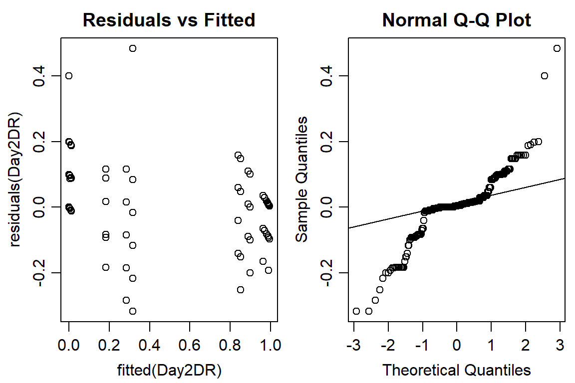
#data not normally distributed

op <- par(mfrow = c(1, 2), mar=c(3.2,3.2,.5,.5), mgp=c(2,.7,0))
plot(Day2DR, broken=TRUE, bty="l", xlab="Conc", ylab="Mortality")
modelFit(Day2DR)
## Goodness-of-fit test
##
## Df Chisq value p value
##
## DRC model 232 71.717 1#model doesn't fit very well, instar doesnt have much effect on DR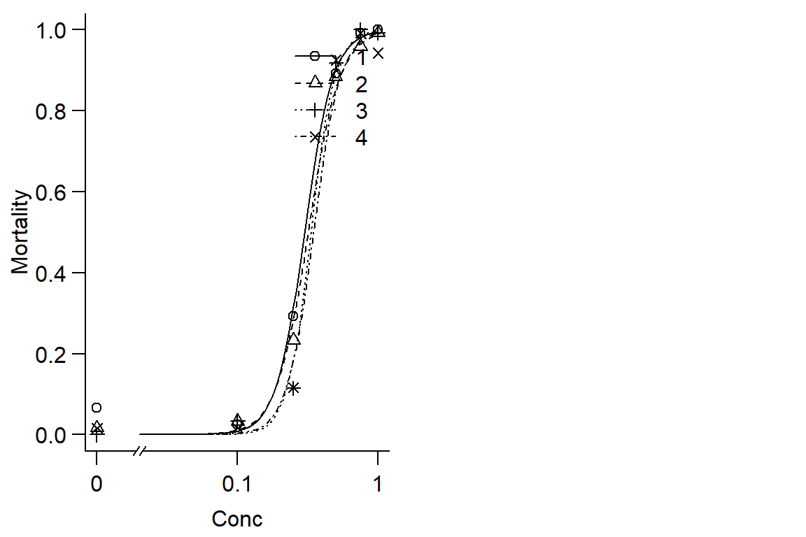
Option 2: Linear Model
#Option 2: look at linear model
pairs(DR$Day2p ~ (DR$Block) + (DR$Rep) + DR$Concentration + DR$Instar)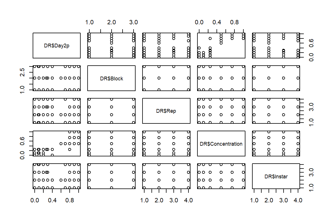
op <- par(mfrow = c(1, 1), mar=c(3.2,3.2,0,.5), mgp=c(2,.7,0))
plot(DR$Day2p ~ DR$Concentration, data = DR, bty="l")
day2.lm <- lm(DR$Day2p ~ (Block) + (Rep) + Concentration + Instar + Concentration:Instar, data = DR)
summary(day2.lm)
##
## Call:
## lm(formula = DR$Day2p ~ (Block) + (Rep) + Concentration + Instar +
## Concentration:Instar, data = DR)
##
## Residuals:
## Min 1Q Median 3Q Max
## -0.35969 -0.16212 -0.02192 0.11120 0.47196
##
## Coefficients:
## Estimate Std. Error t value Pr(>|t|)
## (Intercept) 0.061467 0.057127 1.076 0.283
## Block 0.007197 0.013744 0.524 0.601
## Rep -0.001654 0.010037 -0.165 0.869
## Concentration 1.112013 0.077320 14.382 <2e-16 ***
## Instar -0.021014 0.015825 -1.328 0.185
## Concentration:Instar 0.016180 0.028233 0.573 0.567
## ---
## Signif. codes: 0 '***' 0.001 '**' 0.01 '*' 0.05 '.' 0.1 ' ' 1
##
## Residual standard error: 0.1904 on 282 degrees of freedom
## Multiple R-squared: 0.8257, Adjusted R-squared: 0.8226
## F-statistic: 267.1 on 5 and 282 DF, p-value: < 2.2e-16plot(day2.lm, which=1, bty="l")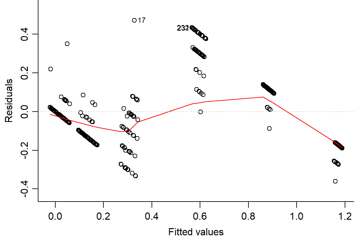
#look at residuals
plot(residuals(day2.lm) ~ fitted(day2.lm), main="Residuals vs Fitted")
abline(h=0) #should look random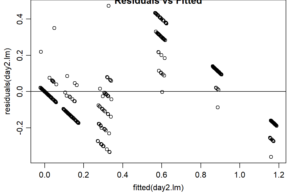
qqnorm(residuals(day2.lm))
qqline(residuals(day2.lm)) 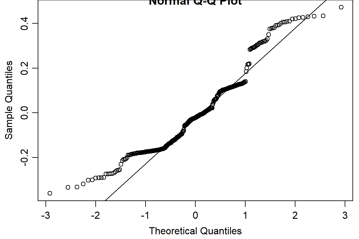
# fit with binomial dist
day2.lm2 <- glm((DR$Day2p)~ (DR$Block) + (DR$Rep) + (DR$Concentration) + (DR$Instar) + (DR$Concentration:DR$Instar), family = binomial(link = "logit"))
## Warning in eval(family$initialize): non-integer #successes in a binomial glm!summary(day2.lm2)##
## Call:
## glm(formula = (DR$Day2p) ~ (DR$Block) + (DR$Rep) + (DR$Concentration) +
## (DR$Instar) + (DR$Concentration:DR$Instar), family = binomial(link = "logit"))
##
## Deviance Residuals:
## Min 1Q Median 3Q Max
## -1.4176 -0.2332 0.0301 0.1454 1.3145
##
## Coefficients:
## Estimate Std. Error z value Pr(>|z|)
## (Intercept) -3.6102 1.4276 -2.529 0.011443 *
## DR$Block 0.1167 0.2910 0.401 0.688496
## DR$Rep -0.0268 0.2122 -0.126 0.899487
## DR$Concentration 11.1180 3.3689 3.300 0.000966 ***
## DR$Instar -0.3291 0.4657 -0.707 0.479807
## DR$Concentration:DR$Instar 0.3105 1.2578 0.247 0.805051
## ---
## Signif. codes: 0 '***' 0.001 '**' 0.01 '*' 0.05 '.' 0.1 ' ' 1
##
## (Dispersion parameter for binomial family taken to be 1)
##
## Null deviance: 313.890 on 287 degrees of freedom
## Residual deviance: 37.273 on 282 degrees of freedom
## AIC: 61.664
##
## Number of Fisher Scoring iterations: 7plot(day2.lm2, which=1, bty="l")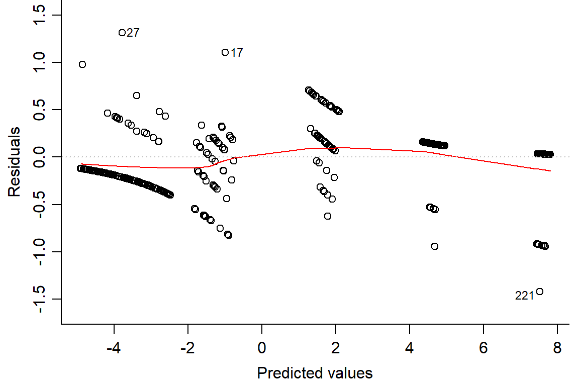
plot(residuals(day2.lm2) ~ fitted(day2.lm2), main="Residuals vs Fitted")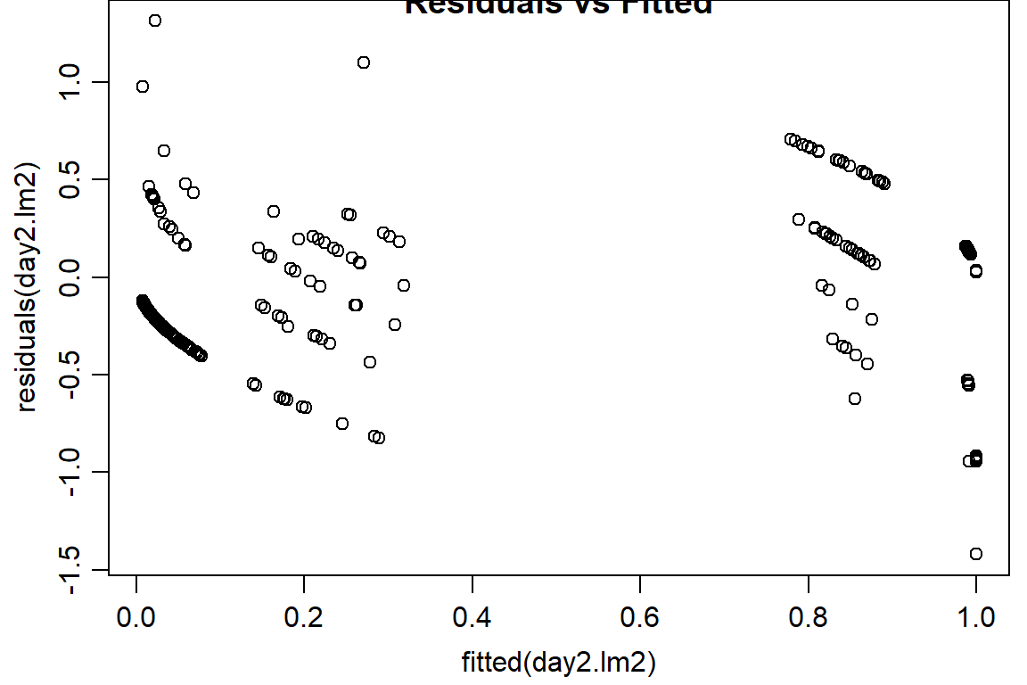
qqnorm(residuals(day2.lm2))
qqline(residuals(day2.lm2)) 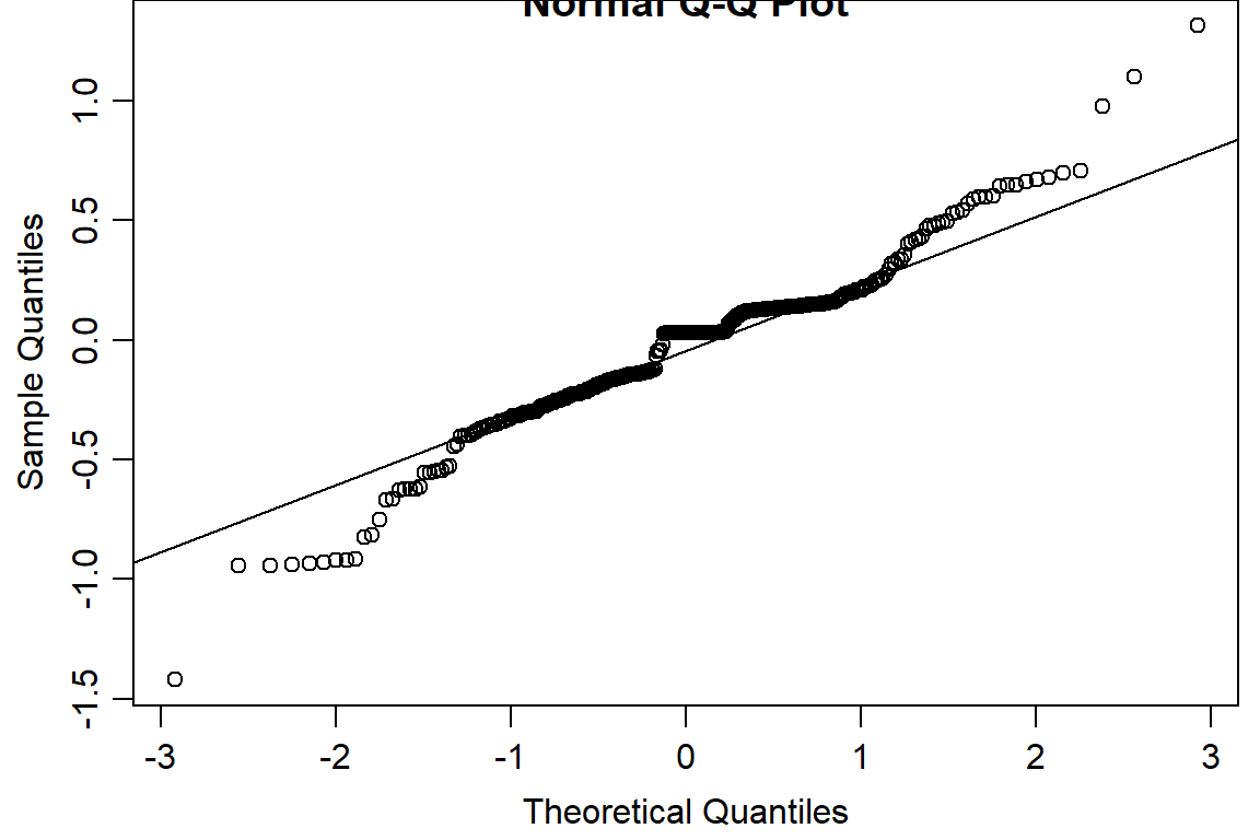
#compare linear model with DR, linear > DR due to lower AIC
AIC(Day2DR, day2.lm, day2.lm2)
## df AIC
## Day2DR 8 189.95387
## day2.lm 7 -129.99081
## day2.lm2 6 61.66438