Background
This example is focued on modeling via linear regression. We will illustrate the concepts using an example, with particular focus on the assumptions and the tools that exist in R to explore the model fit.
Our goal is to related a “dependent variable” with an “independent variable” the explains something about the process.
Our simple example is that we might relate plant height with an index of crop growth (leaf area index). This would provide a simple base for considering in the future the impact of some pest on growth and development.
Our basic model form is: \[Y = f(X) + e\]
Where:
- Y = dependent variable,
- f(X) = a mathematical function that describes the relationship of the dependenct variable as a function of the independent variable,
- e = error, the proper form for a model depends on the type of assumptions; in our simple example, we assume that the error is distributed normally with an expected value of 0 and variance equal to sigma.
For this first example, we are creating a more complete analysis where we will explore some of the tools that help with understanding the model assumptions and also how to use the prediction function, which is important for using the model to estimate new values, as well as information about the variability.
library(tidyverse)
library(Hmisc)
library(corrplot)
library(readr)
library(HH)
library(car)
library(tinytex)
Data
In the majority of our examples, we will use a manual data input approach, to minimize some of the confusion that occurs when trying to import data. R and RStudio are very flexible in this regards.
The data we are using for this first example comes from peanut, where we have two measures: 1. The percentage of clean grain, 2. The concentration of aflatoxin in ppb (ug per kg).
We describe the variables as follows:
- clean = % of clean grain
- aflatoxin = aflatoxin concentration
clean <- c(99.97, 99.94, 99.86, 99.98, 99.93, 99.81, 99.98, 99.91, 99.88, 99.97, 99.97, 99.8, 99.96, 99.99, 99.86, 99.96, 99.93, 99.79, 99.96, 99.86, 99.82, 99.97, 99.99, 99.83, 99.89, 99.96, 99.72, 99.96, 99.91, 99.64, 99.98, 99.86, 99.66, 99.98)
aflatoxin <- c(3, 18.8, 46.8, 4.7, 18.9, 46.8, 8.3, 21.7, 58.1, 9.3, 21.9, 62.3, 9.9, 22.8, 70.6, 11, 24.2, 71.1, 12.3, 25.8, 71.3, 12.5, 30.6, 83.2, 12.6, 36.2, 83.6, 15.9, 39.8, 99.5, 16.7, 44.3, 111.2, 18.8)

peanut <- data.frame(clean, aflatoxin)
head(peanut)
## clean aflatoxin
## 1 99.97 3.0
## 2 99.94 18.8
## 3 99.86 46.8
## 4 99.98 4.7
## 5 99.93 18.9
## 6 99.81 46.8Exploratory analysis
mean(aflatoxin)## [1] 36.60294sd(aflatoxin)## [1] 29.3194sd(aflatoxin)/mean(aflatoxin)*100## [1] 80.1012mean(clean)## [1] 99.89647sd(clean)## [1] 0.09351332sd(clean)/mean(clean)*100## [1] 0.09361024cor(clean, aflatoxin)## [1] -0.9069581rcorr(clean, aflatoxin)## x y
## x 1.00 -0.91
## y -0.91 1.00
##
## n= 34
##
##
## P
## x y
## x 0
## y 0Linear regression
# Visualizing the relationship
with(peanut, plot(x=clean, y=aflatoxin, xlim=c(99.5,100), ylim=c(0,120), pch=10)) 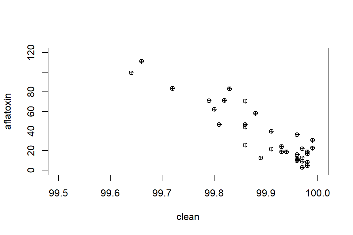
# We will use lm() = linear model, to run the regression

linreg <- with(peanut, lm(aflatoxin~clean)) #Format, Y <- X
anova(linreg) #ANOVA table to see how the model fit looks
## Analysis of Variance Table
##
## Response: aflatoxin
## Df Sum Sq Mean Sq F value Pr(>F)
## clean 1 23334.5 23334.5 148.36 1.479e-13 ***
## Residuals 32 5033.2 157.3
## ---
## Signif. codes: 0 '***' 0.001 '**' 0.01 '*' 0.05 '.' 0.1 ' ' 1summary(linreg) #Another way to see results of the model, with a few more details. This is important as we extend on the modeling concept to understand more complex relationships. ##
## Call:
## lm(formula = aflatoxin ~ clean)
##
## Residuals:
## Min 1Q Median 3Q Max
## -25.843 -7.997 -2.771 6.835 27.695
##
## Coefficients:
## Estimate Std. Error t value Pr(>|t|)
## (Intercept) 28443.18 2332.21 12.20 1.43e-13 ***
## clean -284.36 23.35 -12.18 1.48e-13 ***
## ---
## Signif. codes: 0 '***' 0.001 '**' 0.01 '*' 0.05 '.' 0.1 ' ' 1
##
## Residual standard error: 12.54 on 32 degrees of freedom
## Multiple R-squared: 0.8226, Adjusted R-squared: 0.817
## F-statistic: 148.4 on 1 and 32 DF, p-value: 1.479e-13The results indicated that there is a “significant” relationship. In the next step, we are going to learn about some of the tools that we can use to extract more information about the results to look at hypothesis testing on the parameters (intercept, slope, etc.)
### Example: let's say that we are interested in comparing the slope to a known value of -220, which means that for every 1% change in the percentage of clean grain, the concentration of aflatoxin will be reduced by 220 ug per kg

# First, we need to see and understand where the coefficients are located, especially the intercept and slope
linreg$coef
## (Intercept) clean
## 28443.1778 -284.3601linreg$coef[1]## (Intercept)
## 28443.18linreg$coef[2]## clean
## -284.3601# Furthermore, where are the errors associated with each parameter
coefs <- summary(linreg)
names(coefs)## [1] "call" "terms" "residuals" "coefficients" "aliased" "sigma" "df" "r.squared" "adj.r.squared" "fstatistic" "cov.unscaled"coefs$coefficients## Estimate Std. Error t value Pr(>|t|)
## (Intercept) 28443.1778 2332.20556 12.19583 1.429478e-13
## clean -284.3601 23.34622 -12.18014 1.479070e-13# We can see this directly as follows:
coefs$coefficients[1,1]## [1] 28443.18coefs$coefficients[1,2]## [1] 2332.206coefs$coefficients[2,1]## [1] -284.3601coefs$coefficients[2,2]## [1] 23.34622# Now, we will define the test parameter value for the slope
B1 <- -220
# To realize the test, we need to define the parameter value and the appropriate error term
# abs = absolute value
test_b1<-abs((coefs$coefficients[2,1]-B1)/coefs$coefficients[2,2])
test_b1## [1] 2.75677## Test statistic (two-tailed) with 32 degrees of freedom (error term)
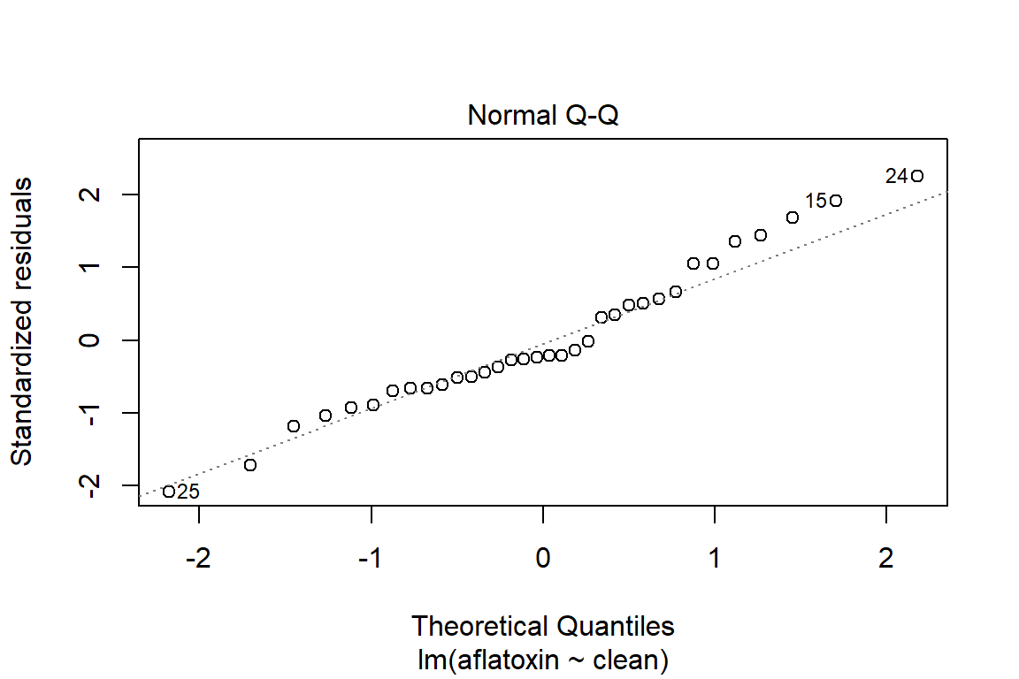
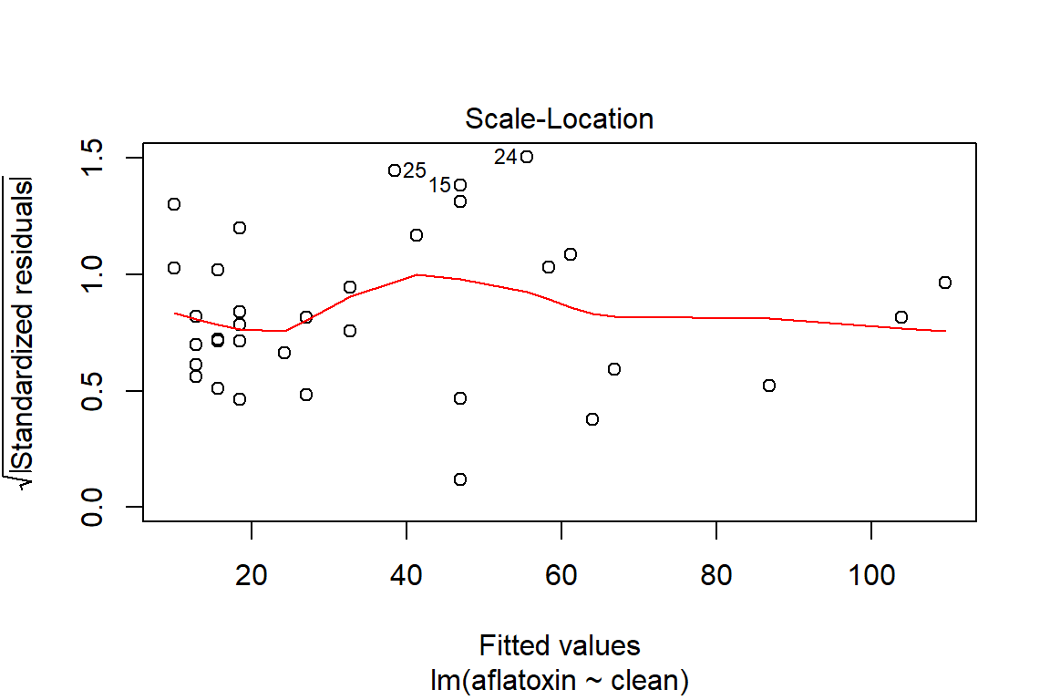
2*pt(q=test_b1, df=32, lower.tail=FALSE) ## [1] 0.009560549Model assumptions
## What does a simple call to plot provide?
plot(linreg)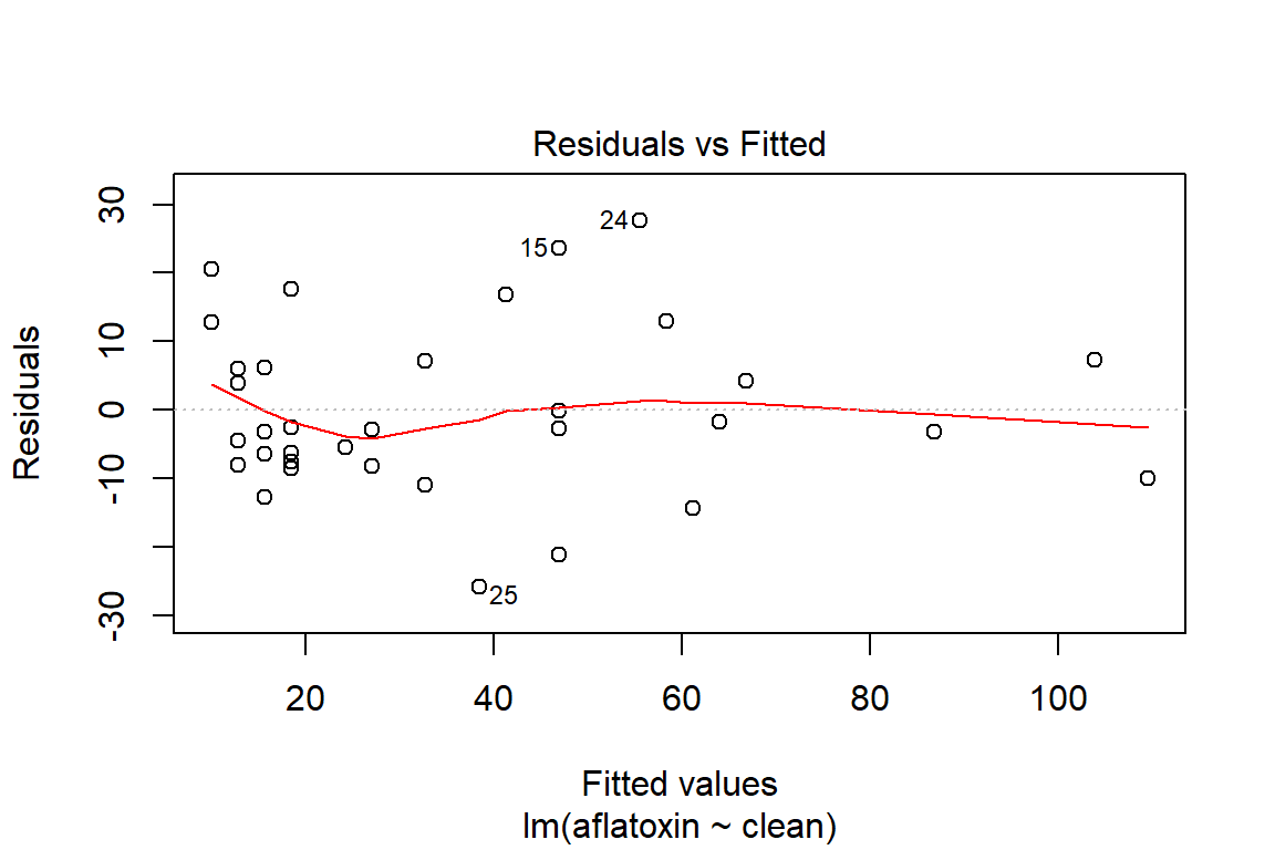
## With Rmarkdown and the reporting tools, we may have interest in controlling the outputted graphics, which can be accomplished as follows:
par(mfrow=c(1,1))
plot(linreg, which=1)
plot(linreg, which=2)
plot(linreg, which=3)
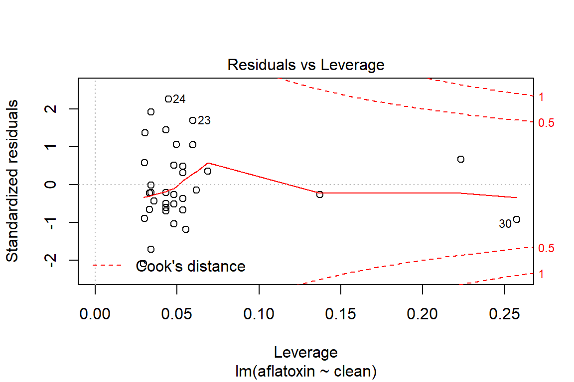
plot(linreg, which=4)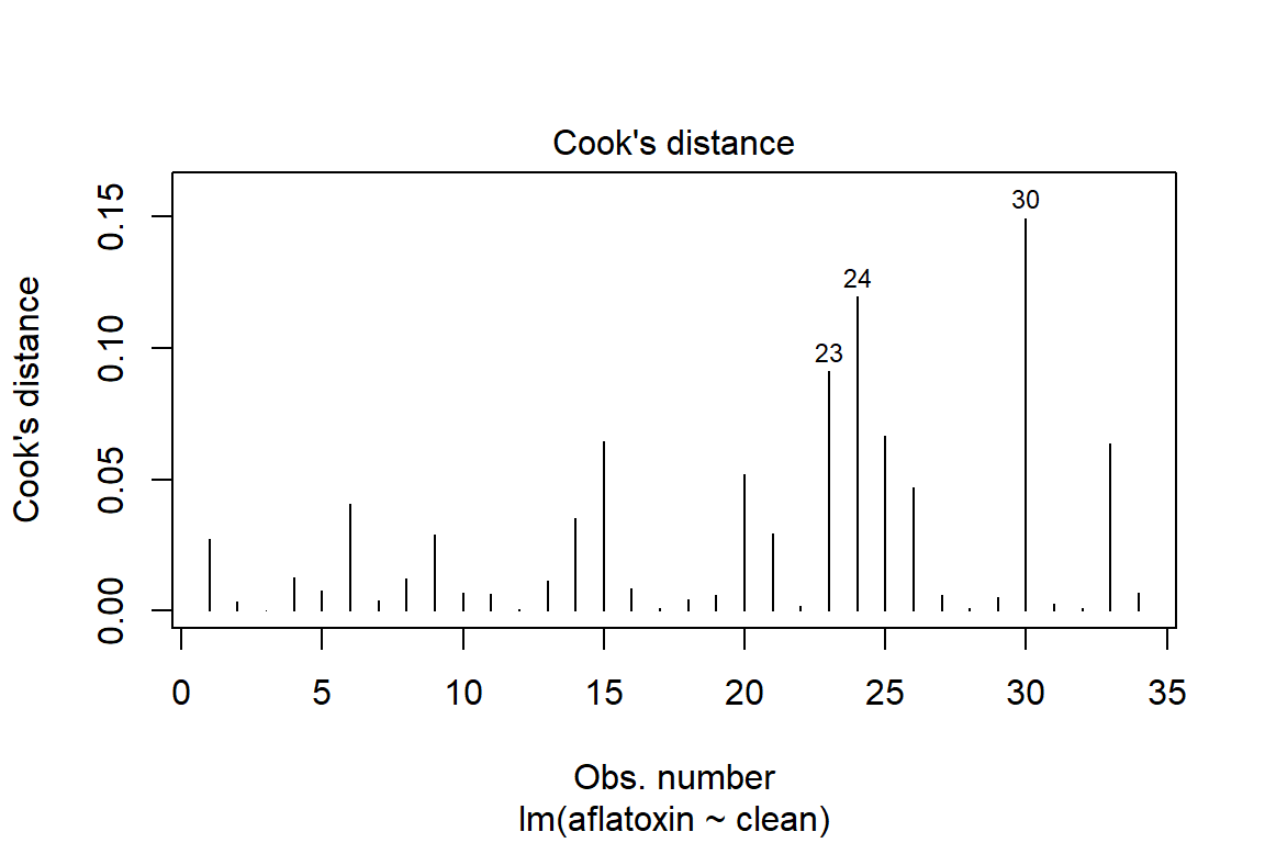
plot(linreg, which=5)
plot(linreg, which=6)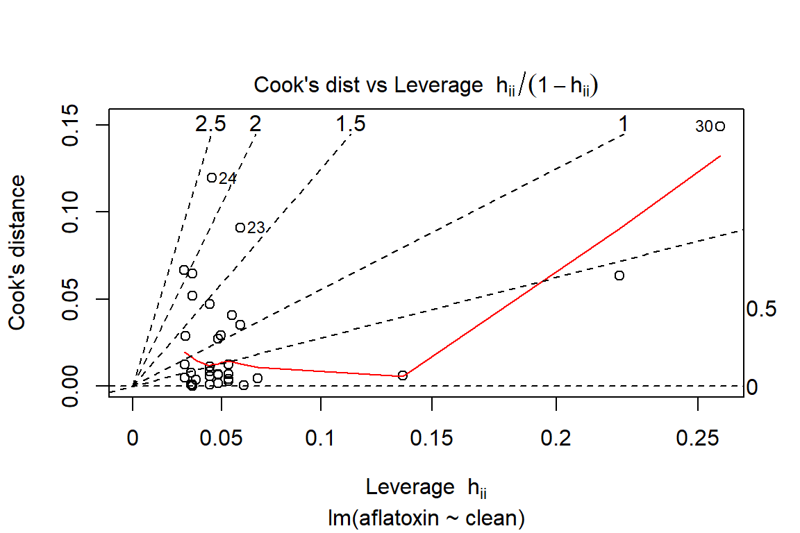
Estimation and prediction
Now that we have a model, we are normally interested in performing some type of prediction based on the model equation (form). In R, the function predict() is very important for many of the modeling tools we might like to apply. This versatile function allows us to perform estimation (within the confines of the model and data structure) and prediction (under uncertainty). What this predicts is the point estimate for a value (or estiamtes for multiple values) as well as the respective interval type (confidence or prediction).
# One challenge with predict is the need to defien a data.frame, even if just for a single value, like the following example where the % clean grain is 99.68.

observation <- data.frame(clean=99.68)

predict(object=linreg, newdata=observation, interval="confidence")
## fit lwr upr
## 1 98.15855 86.97085 109.3462predict(object=linreg, newdata=observation, interval="predict")## fit lwr upr
## 1 98.15855 70.27011 126.047# We can do the same for all values in the regression.
intervals<-predict(linreg, interval="confidence")
intervals## fit lwr upr
## 1 15.69411 10.088679 21.29954
## 2 24.22491 19.379382 29.07044
## 3 46.97372 42.261813 51.68563
## 4 12.85051 6.936739 18.76427
## 5 27.06851 22.406270 31.73076
## 6 61.19173 55.183124 67.20034
## 7 12.85051 6.936739 18.76427
## 8 32.75572 28.327614 37.18382
## 9 41.28652 36.835944 45.73710
## 10 15.69411 10.088679 21.29954
## 11 15.69411 10.088679 21.29954
## 12 64.03533 57.691794 70.37887
## 13 18.53771 13.215931 23.85949
## 14 10.00690 3.763770 16.25004
## 15 46.97372 42.261813 51.68563
## 16 18.53771 13.215931 23.85949
## 17 27.06851 22.406270 31.73076
## 18 66.87893 60.183421 73.57445
## 19 18.53771 13.215931 23.85949
## 20 46.97372 42.261813 51.68563
## 21 58.34813 52.654402 64.04186
## 22 15.69411 10.088679 21.29954
## 23 10.00690 3.763770 16.25004
## 24 55.50453 50.102122 60.90693
## 25 38.44292 34.051014 42.83482
## 26 18.53771 13.215931 23.85949
## 27 86.78414 77.317367 96.25092
## 28 18.53771 13.215931 23.85949
## 29 32.75572 28.327614 37.18382
## 30 109.53295 96.573565 122.49234
## 31 12.85051 6.936739 18.76427
## 32 46.97372 42.261813 51.68563
## 33 103.84575 91.777175 115.91433
## 34 12.85051 6.936739 18.76427predictions<-predict(linreg, interval="predict")## Warning in predict.lm(linreg, interval = "predict"): predictions on current data refer to _future_ responsespredictions## fit lwr upr
## 1 15.69411 -10.459699 41.84791
## 2 24.22491 -1.776625 50.22645
## 3 46.97372 20.996756 72.95069
## 4 12.85051 -13.371114 39.07213
## 5 27.06851 1.100509 53.03652
## 6 61.19173 34.948558 87.43490
## 7 12.85051 -13.371114 39.07213
## 8 32.75572 6.828726 58.68271
## 9 41.28652 15.355682 67.21736
## 10 15.69411 -10.459699 41.84791
## 11 15.69411 -10.459699 41.84791
## 12 64.03533 37.713455 90.35721
## 13 18.53771 -7.556774 44.63219
## 14 10.00690 -16.290956 36.30476
## 15 46.97372 20.996756 72.95069
## 16 18.53771 -7.556774 44.63219
## 17 27.06851 1.100509 53.03652
## 18 66.87893 40.470022 93.28784
## 19 18.53771 -7.556774 44.63219
## 20 46.97372 20.996756 72.95069
## 21 58.34813 32.175256 84.52100
## 22 15.69411 -10.459699 41.84791
## 23 10.00690 -16.290956 36.30476
## 24 55.50453 29.393482 81.61557
## 25 38.44292 12.522086 64.36375
## 26 18.53771 -7.556774 44.63219
## 27 86.78414 59.540418 114.02787
## 28 18.53771 -7.556774 44.63219
## 29 32.75572 6.828726 58.68271
## 30 109.53295 80.887772 138.17814
## 31 12.85051 -13.371114 39.07213
## 32 46.97372 20.996756 72.95069
## 33 103.84575 75.592411 132.09909
## 34 12.85051 -13.371114 39.07213# If we are interested in just some select values, it is easy to accomplish this going back to the original single value example:
observations <- data.frame(clean=c(99.5, 99.6, 99.7, 99.8))
predict(object=linreg, newdata=observations, interval="confidence")## fit lwr upr
## 1 149.34338 129.98701 168.69974
## 2 120.90736 106.14377 135.67095
## 3 92.47135 82.15206 102.79063
## 4 64.03533 57.69179 70.37887predict(object=linreg, newdata=observations, interval="predict")## fit lwr upr
## 1 149.34338 117.29233 181.39442
## 2 120.90736 91.40203 150.41269
## 3 92.47135 64.91979 120.02290
## 4 64.03533 37.71345 90.35721Additional material
The package HH (Statistical analysis and data display, https://www.amazon.com/Statistical-Analysis-Data-Display-Intermediate/dp/1493921215) has various (interesting) functions that we can use to examine a regression model. In the next section, we will look at several of those.
# Let's examine the regression graphically
ci.plot(linreg)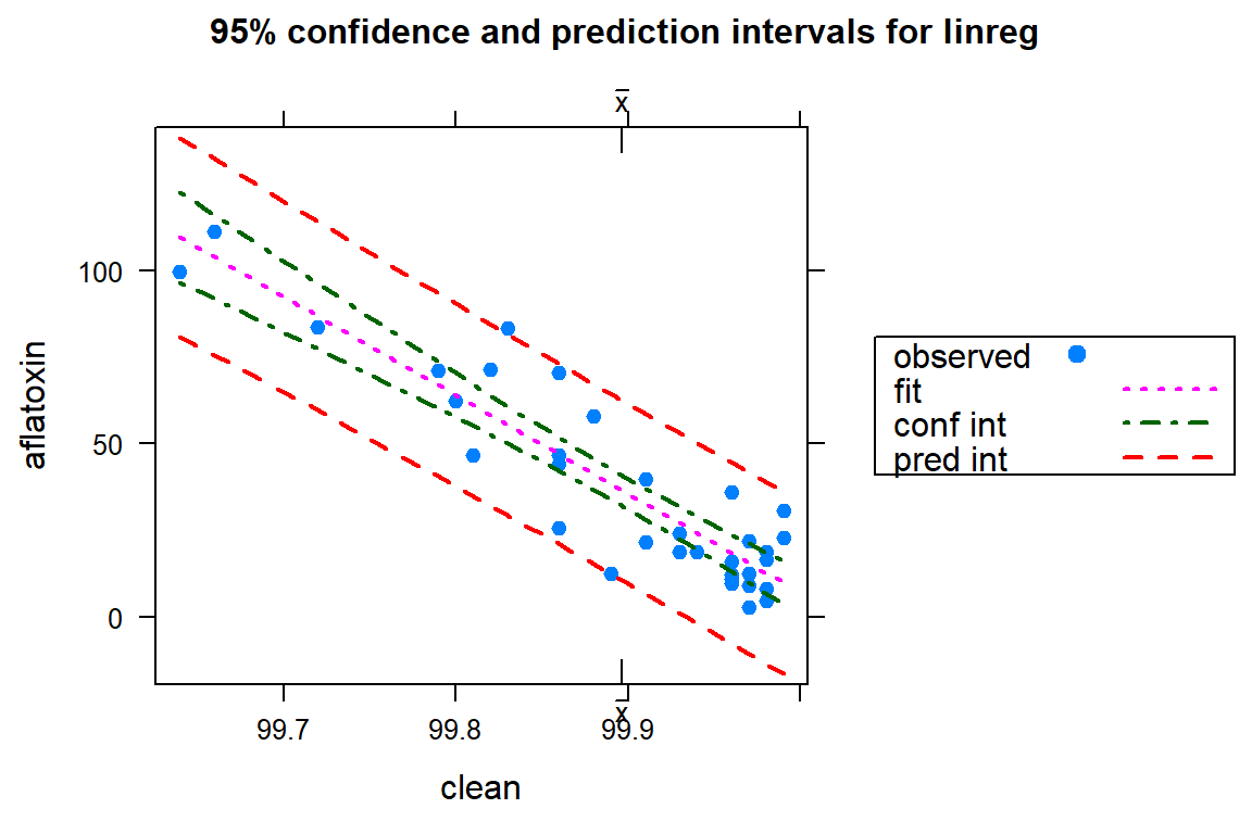
# Tools to study the assumptions

# Method to look for outliers using a Bonferroni adjustment
outlierTest(linreg)
## No Studentized residuals with Bonferroni p < 0.05
## Largest |rstudent|:
## rstudent unadjusted p-value Bonferroni p
## 24 2.425727 0.021292 0.72394# Quantile-quantile plot based on Student residuals
qqPlot(linreg) 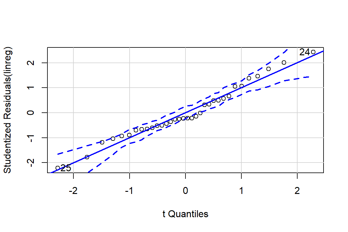
## [1] 24 25# Influence plot in which the size of the circle is proportion to Cook's distance
influencePlot(linreg) 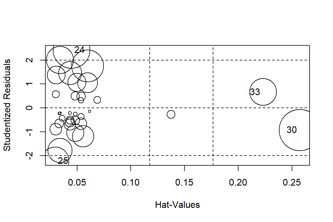
##       StudRes        Hat      CookD
## 24  2.4257274 0.04472257 0.11949821
## 25 -2.2158610 0.02955685 0.06663113
## 30 -0.9262390 0.25734844 0.14930872
## 33  0.6594215 0.22318480 0.06358898
# Test of homoscedasticity
ncvTest(linreg)## Non-constant Variance Score Test
## Variance formula: ~ fitted.values
## Chisquare = 0.183475, Df = 1, p = 0.6684# Method to verify if there is dependency in the model, which means that a transformation may be appropriate to model the relationship
spreadLevelPlot(linreg) 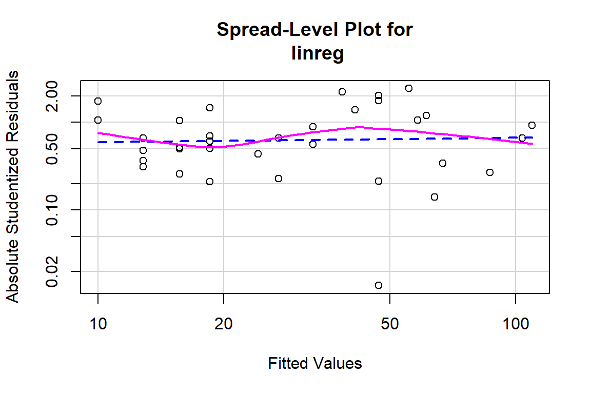
##
## Suggested power transformation:  0.9466765
# Method to verify if there is evidence that the relationship is not linear
crPlots(linreg)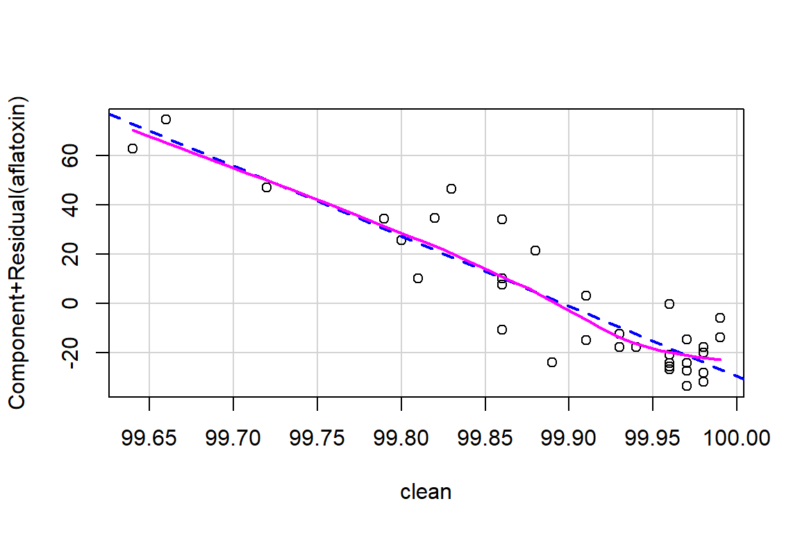
Summary
In this exercise, the goal was to introduce different concepts in modeling, using a simple linear regression. With this base, we will extend the modeling idea with different examples that illustrate some of the tools that exist in R when we have more complex relationships. Given the time available for this workshop, even if the subsequent examples are more difficult to understand, this first, more developed example hopefully provides you some of the relevant tools to take the next step in your work to define and use different models. .
Example
The below example looks at the relationship between the weight of chickens as a function of the amount of lysine, which is an essential amino acid in the early phases of development.
weight <-c(14.7, 17.8, 19.6, 18.4, 20.5, 21.1, 17.2, 18.7, 20.2, 16.0, 17.8, 19.4)
lysine <-c(0.09, 0.14, 0.18, 0.15, 0.16, 0.23, 0.11, 0.19, 0.23, 0.13, 0.17, 0.21)