Background
Given the background and tools presented in linear regression, we will not extend the modeling approach to include additional variables, as well as relationships that are more complicated. This exercise provides the jumping off point for more automated modeling approaches, which will we see in the subsequent example(s).
Our assumption in this exercise is that multiple factors have explanatory value to explain the response variable of interest.
What does a model of this type look like? Some examples include:
- Additive.
\(Y = \beta_0 + \beta_1{X_1} + \beta_2{X_2} + \epsilon\)
- With interaction between the two terms.
\(Y = \beta_0 + \beta_1{X_1} + \beta_2{X_2} + \beta_3{X_1}{X_2} + \epsilon\)
Note: It is important to note that in modeling, when we add new explanatory variables that have merit (i.e., the sign makes sense in terms of the biological relation), the model will improve. This is not necessarily the same as being “biologically relevant”. We should always consider the variable in the context of the question of interest.
library(tidyverse)
library(Hmisc)
library(corrplot)
library(readr)
library(HH)
library(car)
library(scatterplot3d)
library(olsrr)
Data and exploratory analysis
Our database comes from counts of the number of aphids in different lots, as well as measures of average temperature and relative humidity. We assume that there is a relationship between those two latter factors with the observed number of aphids, which means from a predictive value, we hope that by just measuring T and RH, we can estimate the number of expected aphids.
Where do we start? The main question is to determine if there is (are) a relationship between T and RH with the counts. We are also interested in trying to determine if there may be a complext relationship (i.e., that the predictive values have some degree of interpretable interaction).
lot <- c(1:34)
aphids <- c(61, 77, 87, 93, 98, 100, 104, 118, 102, 74, 63, 43, 27, 19, 14, 23, 30, 25, 67, 40, 6, 21, 18, 23, 42, 56, 60, 59, 82, 89, 77, 102, 108, 97)
temperature <- c(21, 24.8, 28.3, 26, 27.5, 27.1, 26.8, 29, 28.3, 34, 30.5, 28.3, 30.8, 31, 33.6, 31.8, 31.3, 33.5, 33, 34.5, 34.3, 34.3, 33, 26.5, 32, 27.3, 27.8, 25.8, 25, 18.5, 26, 19, 18, 16.3)
humidity <- c(57,48, 41.5, 56, 58, 31, 36.5, 41, 40, 25, 34, 13, 37, 19, 20, 17, 21, 18.5, 24.5, 16, 6, 26, 21, 26, 28, 24.5, 39, 29, 41, 53.5, 51, 48, 70, 79.5)

aphids_data <- data.frame(lot, aphids, temperature, humidity)

# Quick exploratory analysis
summary(aphids_data)
## lot aphids temperature humidity
## Min. : 1.00 Min. : 6.00 Min. :16.30 Min. : 6.00
## 1st Qu.: 9.25 1st Qu.: 27.75 1st Qu.:26.00 1st Qu.:21.88
## Median :17.50 Median : 62.00 Median :28.30 Median :32.50
## Mean :17.50 Mean : 61.91 Mean :28.09 Mean :35.19
## 3rd Qu.:25.75 3rd Qu.: 92.00 3rd Qu.:31.95 3rd Qu.:46.38
## Max. :34.00 Max. :118.00 Max. :34.50 Max. :79.50cor(aphids_data[,2:4])## aphids temperature humidity
## aphids 1.0000000 -0.6463022 0.7394570
## temperature -0.6463022 1.0000000 -0.8313696
## humidity 0.7394570 -0.8313696 1.0000000plot(aphids_data[,2:4]) # Graphical matrix
pairs(aphids_data[,2:4]) # Gives us the same thing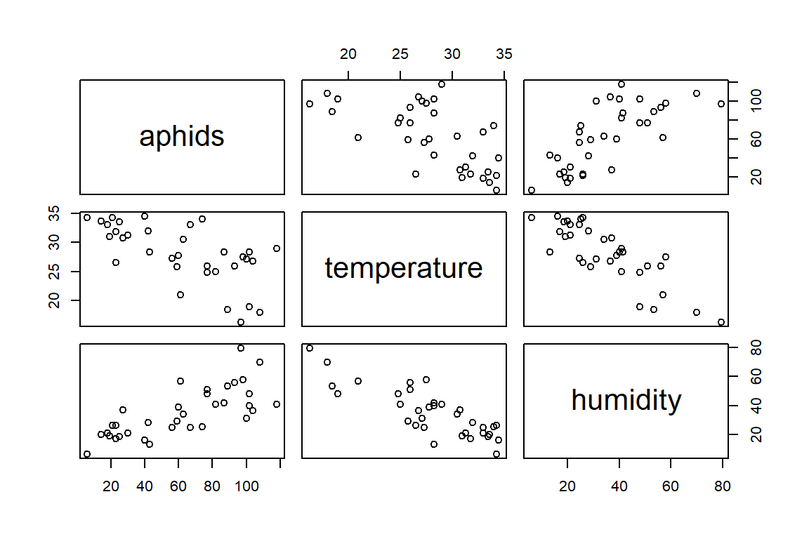
Linear regression
# Factor = temperature (X)
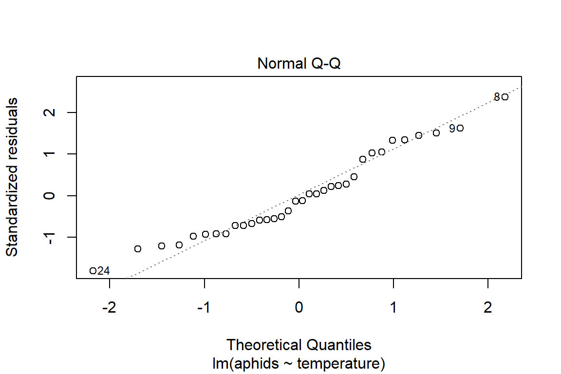
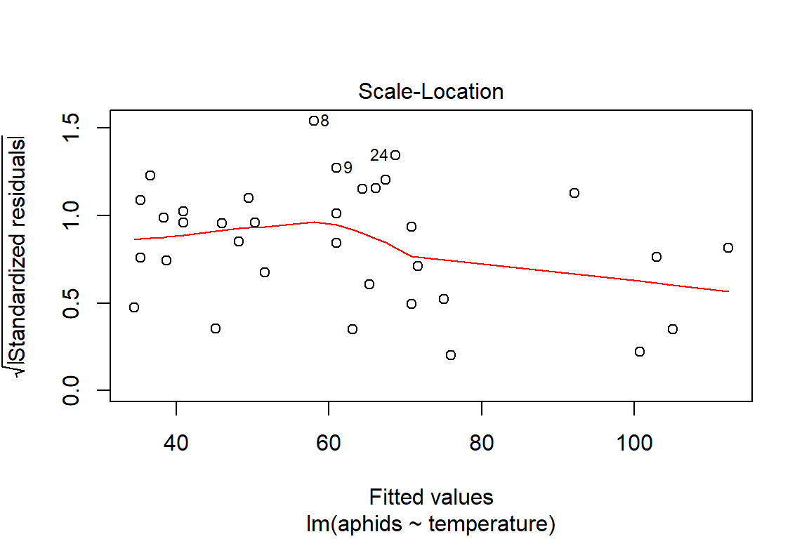
model1<-with(aphids_data, lm(aphids~temperature))
anova(model1)## Analysis of Variance Table
##
## Response: aphids
## Df Sum Sq Mean Sq F value Pr(>F)
## temperature 1 15195 15194.8 22.955 3.643e-05 ***
## Residuals 32 21182 661.9
## ---
## Signif. codes: 0 '***' 0.001 '**' 0.01 '*' 0.05 '.' 0.1 ' ' 1summary(model1)##
## Call:
## lm(formula = aphids ~ temperature)
##
## Residuals:
## Min 1Q Median 3Q Max
## -45.698 -18.111 -3.143 19.477 60.004
##
## Coefficients:
## Estimate Std. Error t value Pr(>|t|)
## (Intercept) 182.1386 25.4785 7.149 4.10e-08 ***
## temperature -4.2808 0.8935 -4.791 3.64e-05 ***
## ---
## Signif. codes: 0 '***' 0.001 '**' 0.01 '*' 0.05 '.' 0.1 ' ' 1
##
## Residual standard error: 25.73 on 32 degrees of freedom
## Multiple R-squared: 0.4177, Adjusted R-squared: 0.3995
## F-statistic: 22.96 on 1 and 32 DF, p-value: 3.643e-05plot(model1)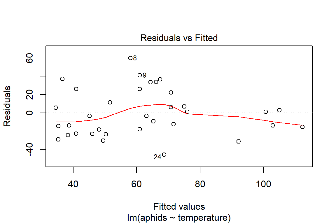
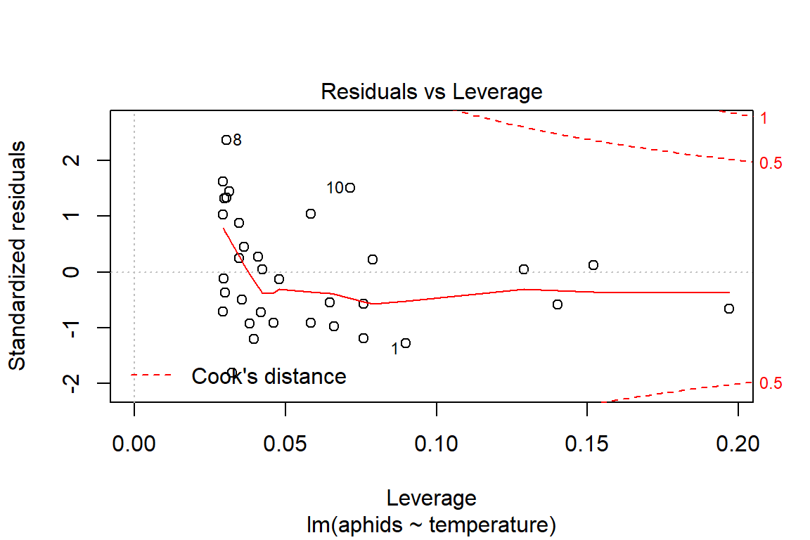
# Assumptions = values, model1

rstudent(model1)
## 1 2 3 4 5 6 7 8 9 10 11 12 13 14 15 16 17 18 19 20 21 22 23 24 25 26 27 28 29 30 31 32 33 34
## -1.28585895 0.04005818 1.02696012 0.87344711 1.34166917 1.35439948 1.47093718 2.56708773 1.66182645 1.54106791 0.44669460 -0.70426322 -0.92092001 -1.21610745 -0.97682293 -0.91330799 -0.71519631 -0.54584549 1.04821427 0.22134400 -1.19286546 -0.57242992 -0.91388994 -1.87539948 -0.12367881 -0.36099265 -0.12169500 -0.49651581 0.26909704 -0.57840180 0.24013268 0.04903167 0.12114783 -0.66038629dfbetas(model1)## (Intercept) temperature
## 1 -0.366682839 0.331661207
## 2 0.005815635 -0.004670407
## 3 0.023305013 0.007772618
## 4 0.089808162 -0.064378045
## 5 0.067723562 -0.027686588
## 6 0.087212625 -0.047068694
## 7 0.110092705 -0.066711426
## 8 -0.004133934 0.082814320
## 9 0.037712163 0.012577648
## 10 -0.276055170 0.328520764
## 11 -0.024068323 0.038160258
## 12 -0.015981987 -0.005330265
## 13 0.059303647 -0.088531881
## 14 0.086856812 -0.125611236
## 15 0.160634492 -0.193579923
## 16 0.091034920 -0.120629792
## 17 0.058637009 -0.081569976
## 18 0.087768241 -0.106135446
## 19 -0.149512336 0.184383492
## 20 -0.043753984 0.051380499
## 21 0.226920851 -0.267823576
## 22 0.108894329 -0.128522648
## 23 0.130352947 -0.160755509
## 24 -0.160003296 0.104963953
## 25 0.013206774 -0.017231640
## 26 -0.020732461 0.009996651
## 27 -0.004874275 0.001223897
## 28 -0.054538615 0.040127888
## 29 0.037156513 -0.029440595
## 30 -0.223031160 0.207642177
## 31 0.024690533 -0.017699151
## 32 0.017885539 -0.016575675
## 33 0.049290028 -0.046078814
## 34 -0.318930693 0.301601424dffits(model1)## 1 2 3 4 5 6 7 8 9 10 11 12 13 14 15 16 17 18 19 20 21 22 23 24 25 26 27 28 29 30 31 32 33 34
## -0.404272806 0.008432063 0.178944815 0.165495030 0.235239322 0.240562702 0.264859612 0.454709984 0.289568427 0.427975171 0.086872782 -0.122715819 -0.183780341 -0.247127470 -0.259852603 -0.200671906 -0.149517430 -0.143648162 0.261386769 0.064842854 -0.342084958 -0.164159053 -0.227891133 -0.343410519 -0.027739070 -0.063654708 -0.021220776 -0.095548871 0.055563960 -0.233580039 0.045498765 0.018866121 0.051306429 -0.327009697covratio(model1)## 1 2 3 4 5 6 7 8 9 10 11 12 13 14 15 16 17 18 19 20 21 22 23 24 25 26 27 28 29 30 31 32 33 34
## 1.0553084 1.1126545 1.0268519 1.0514226 0.9810703 0.9797855 0.9612415 0.7474350 0.9256398 0.9902076 1.0917586 1.0636026 1.0497679 1.0108127 1.0738384 1.0592292 1.0763152 1.1177641 1.0556567 1.1533544 1.0541908 1.1291908 1.0732083 0.8882885 1.1180537 1.0895089 1.0969090 1.0876492 1.1058148 1.2130097 1.0997154 1.2231239 1.2554800 1.2902753cooks.distance(model1)## 1 2 3 4 5 6 7 8 9 10 11 12 13 14 15 16 17 18 19 20 21 22 23 24 25 26 27 28 29 30 31 32 33 34
## 8.008297e-02 3.669472e-05 1.598333e-02 1.379652e-02 2.699386e-02 2.819990e-02 3.384457e-02 8.800702e-02 3.973731e-02 8.780865e-02 3.870253e-03 7.650078e-03 1.696816e-02 3.008573e-02 3.381010e-02 2.023952e-02 1.135101e-02 1.054883e-02 3.405642e-02 2.166690e-03 5.774783e-02 1.376327e-02 2.610161e-02 5.466541e-02 3.969427e-04 2.082560e-03 2.323129e-04 4.674868e-03 1.589759e-03 2.785916e-02 1.066474e-03 1.836918e-04 1.357989e-03 5.442676e-02# Factor = humedad (X)
model2<-with(aphids_data, lm(aphids~humidity))
anova(model2)## Analysis of Variance Table
##
## Response: aphids
## Df Sum Sq Mean Sq F value Pr(>F)
## humidity 1 19891 19890.7 38.608 5.857e-07 ***
## Residuals 32 16486 515.2
## ---
## Signif. codes: 0 '***' 0.001 '**' 0.01 '*' 0.05 '.' 0.1 ' ' 1summary(model2)##
## Call:
## lm(formula = aphids ~ humidity)
##
## Residuals:
## Min 1Q Median 3Q Max
## -37.53 -13.44 -1.43 12.82 47.68
##
## Coefficients:
## Estimate Std. Error t value Pr(>|t|)
## (Intercept) 10.9787 9.0744 1.210 0.235
## humidity 1.4473 0.2329 6.214 5.86e-07 ***
## ---
## Signif. codes: 0 '***' 0.001 '**' 0.01 '*' 0.05 '.' 0.1 ' ' 1
##
## Residual standard error: 22.7 on 32 degrees of freedom
## Multiple R-squared: 0.5468, Adjusted R-squared: 0.5326
## F-statistic: 38.61 on 1 and 32 DF, p-value: 5.857e-07plot(model2)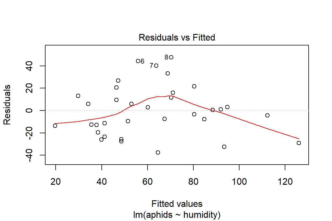
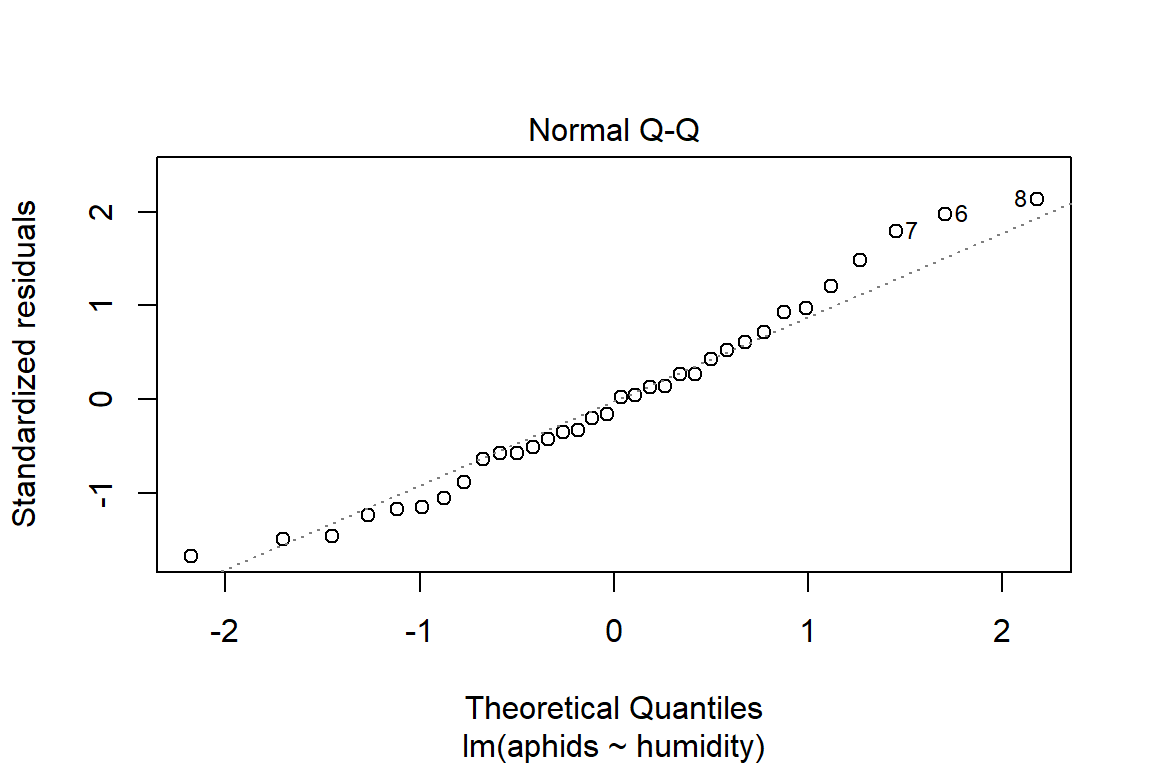
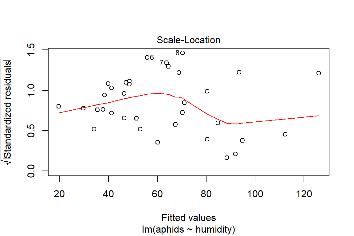
# Assumptions = values, model2

rstudent(model2)
## 1 2 3 4 5 6 7 8 9 10 11 12 13 14 15 16 17 18 19 20 21 22 23 24 25 26 27 28 29 30 31 32 33 34
## -1.52166116 -0.15329366 0.70958337 0.04378704 0.13944816 2.07616739 1.86604477 2.27067980 1.51293060 1.21600986 0.12382267 0.60092052 -1.73010695 -0.88059890 -1.18139920 -0.56699356 -0.50823171 -0.57307681 0.92313524 0.26372262 -0.63535605 -1.25128763 -1.05882161 -1.15657354 -0.42068829 0.42473282 -0.32760978 0.26710592 0.51730586 0.02642984 -0.34840648 0.97153856 -0.20281479 -1.49172395dfbetas(model2)## (Intercept) humidity
## 1 0.203962802 -0.354960067
## 2 0.007091915 -0.020637509
## 3 0.010888321 0.046732070
## 4 -0.005432893 0.009722237
## 5 -0.020090271 0.034108001
## 6 0.237139151 -0.090726882
## 7 0.116375070 0.025442918
## 8 0.045533868 0.137646115
## 9 0.044574968 0.075879906
## 10 0.208590411 -0.129821254
## 11 0.010635007 -0.001536502
## 12 0.175091541 -0.142772652
## 13 -0.099765368 -0.032603908
## 14 -0.202822717 0.150676741
## 15 -0.260370374 0.189329385
## 16 -0.141963444 0.109421496
## 17 -0.106991971 0.075962840
## 18 -0.134852336 0.101178572
## 19 0.162812727 -0.103448492
## 20 0.068702630 -0.053805692
## 21 -0.232992130 0.202795860
## 22 -0.202585666 0.120351428
## 23 -0.222901106 0.158256745
## 24 -0.187251287 0.111241631
## 25 -0.060049112 0.031601350
## 26 0.074909835 -0.047596460
## 27 -0.012732795 -0.013008080
## 28 0.035580371 -0.017261761
## 29 0.010373518 0.031358513
## 30 -0.002627836 0.005134802
## 31 0.026166587 -0.058167303
## 32 -0.044946864 0.130795599
## 33 0.055027998 -0.078907786
## 34 0.575503750 -0.776106220dffits(model2)## 1 2 3 4 5 6 7 8 9 10 11 12 13 14 15 16 17 18 19 20 21 22 23 24 25 26 27 28 29 30 31 32 33 34
## -0.447191192 -0.033924951 0.132317421 0.012469416 0.042283274 0.372962648 0.325861688 0.419240517 0.274398674 0.249344653 0.021611110 0.178729735 -0.302985776 -0.216541182 -0.281470975 -0.148585846 -0.117356163 -0.143175941 0.191962176 0.071346658 -0.233677243 -0.249738808 -0.244493286 -0.230835253 -0.079949336 0.088321443 -0.058538076 0.049688881 0.095511299 0.006952189 -0.084642540 0.215008230 -0.087530558 -0.829472811covratio(model2)## 1 2 3 4 5 6 7 8 9 10 11 12 13 14 15 16 17 18 19 20 21 22 23 24 25 26 27 28 29 30 31 32 33 34
## 1.0022713 1.1160516 1.0676446 1.1518269 1.1620673 0.8477864 0.8874781 0.8100232 0.9544553 1.0115565 1.0969300 1.1332631 0.9133416 1.0755087 1.0311057 1.1154780 1.1038994 1.1084567 1.0529470 1.1384310 1.1787935 1.0040208 1.0453923 1.0182323 1.0915424 1.0988072 1.0920026 1.0973744 1.0831002 1.1392331 1.1196610 1.0526653 1.2606798 1.2144142cooks.distance(model2)## 1 2 3 4 5 6 7 8 9 10 11 12 13 14 15 16 17 18 19 20 21 22 23 24 25 26 27 28 29 30 31 32 33 34
## 9.604190e-02 5.935641e-04 8.891911e-03 8.024605e-05 9.221958e-04 6.302998e-02 4.927114e-02 7.777970e-02 3.618960e-02 3.062822e-02 2.409338e-04 1.629755e-02 4.320873e-02 2.361072e-02 3.912909e-02 1.127801e-02 7.049632e-03 1.046940e-02 1.851025e-02 2.621394e-03 2.782097e-02 3.064301e-02 2.977580e-02 2.636426e-02 3.280316e-03 4.002862e-03 1.762520e-03 1.271389e-03 4.668043e-03 2.494547e-05 3.683311e-03 2.315487e-02 3.949133e-03 3.313265e-01Additive multiple regression
Model form:
\[aphids = intercept + temperature + humidity + error\]
model3<-with(aphids_data, lm(aphids~temperature+humidity))
anova(model3)
## Analysis of Variance Table
##
## Response: aphids
## Df Sum Sq Mean Sq F value Pr(>F)
## temperature 1 15194.8 15194.8 28.7765 7.554e-06 ***
## humidity 1 4813.1 4813.1 9.1151 0.005038 **
## Residuals 31 16368.9 528.0
## ---
## Signif. codes: 0 '***' 0.001 '**' 0.01 '*' 0.05 '.' 0.1 ' ' 1summary(model3)##
## Call:
## lm(formula = aphids ~ temperature + humidity)
##
## Residuals:
## Min 1Q Median 3Q Max
## -35.393 -14.006 -3.198 10.335 49.265
##
## Coefficients:
## Estimate Std. Error t value Pr(>|t|)
## (Intercept) 35.8255 53.5388 0.669 0.50835
## temperature -0.6765 1.4360 -0.471 0.64089
## humidity 1.2811 0.4243 3.019 0.00504 **
## ---
## Signif. codes: 0 '***' 0.001 '**' 0.01 '*' 0.05 '.' 0.1 ' ' 1
##
## Residual standard error: 22.98 on 31 degrees of freedom
## Multiple R-squared: 0.55, Adjusted R-squared: 0.521
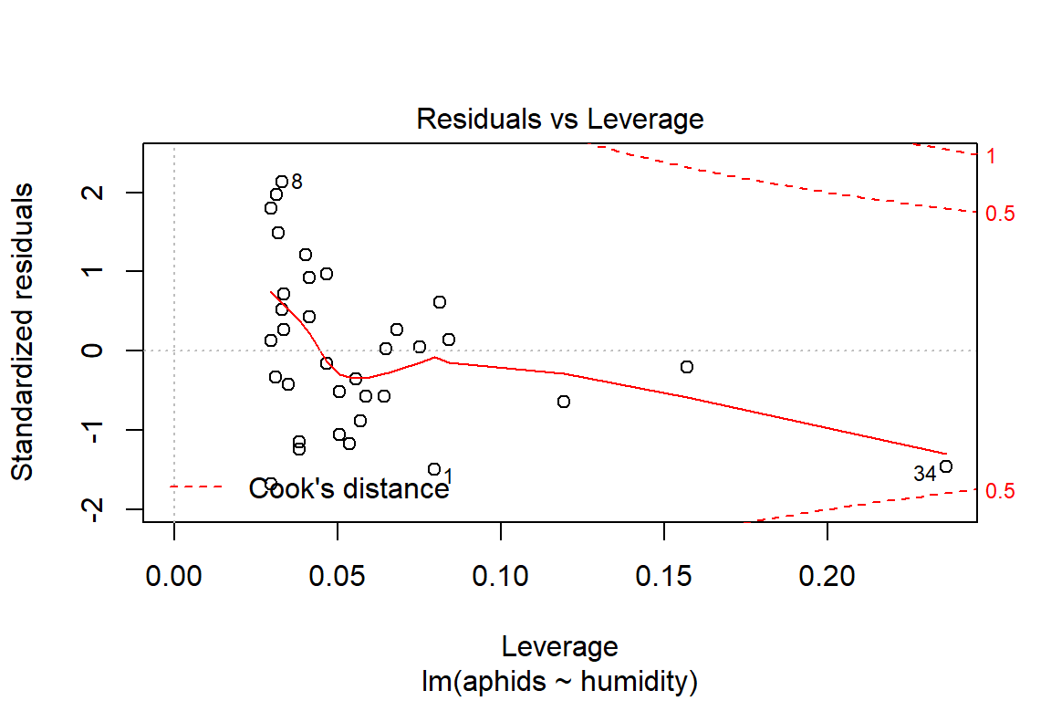
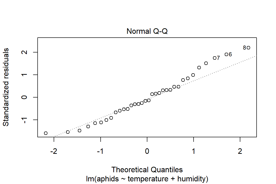
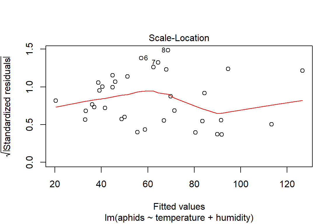
## F-statistic: 18.95 on 2 and 31 DF, p-value: 4.212e-06plot(model3)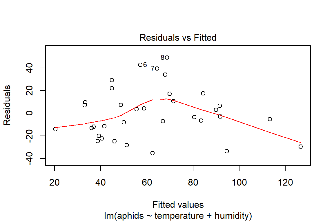
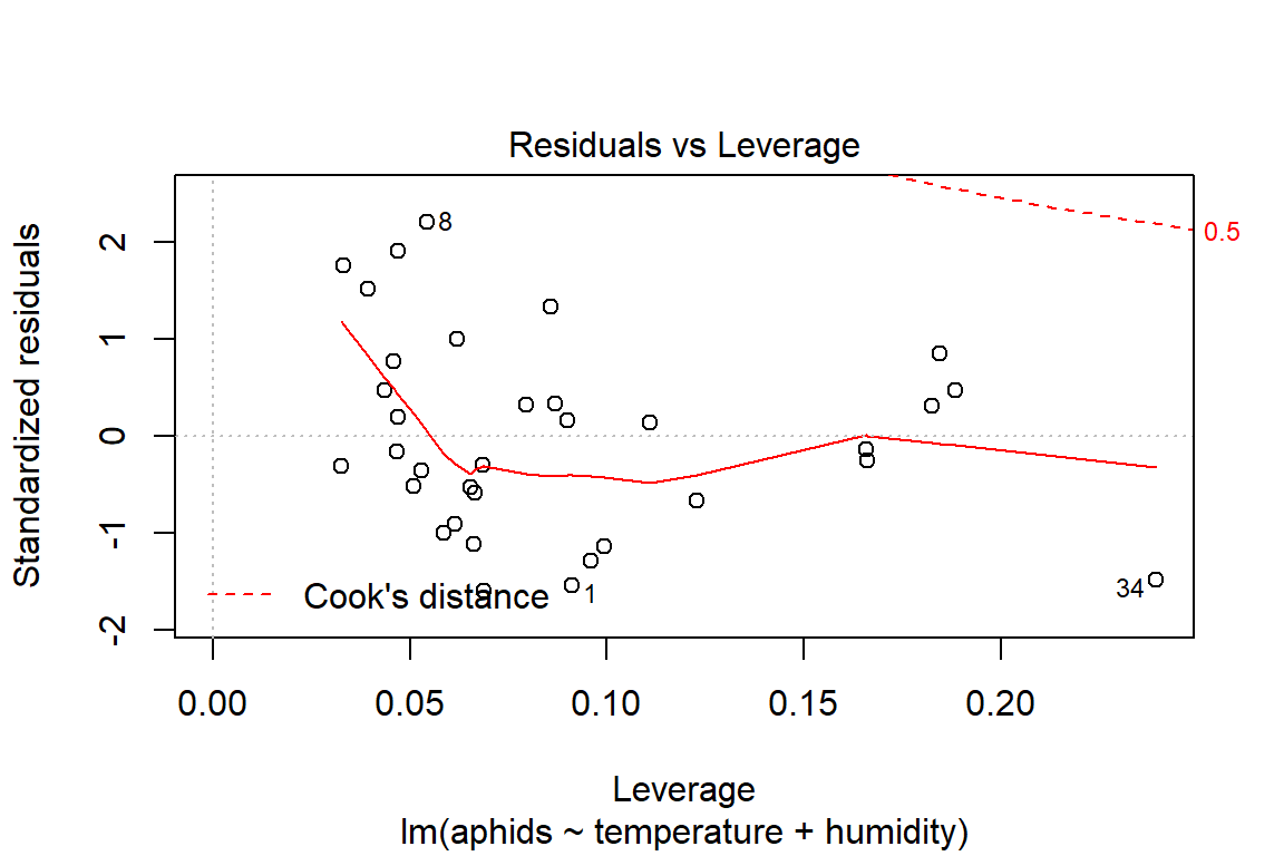
vif(lm(aphids~temperature+humidity, data=aphids_data))## temperature humidity
## 3.238084 3.238084# Assumptions = values, model3
rstudent(model3)## 1 2 3 4 5 6 7 8 9 10 11 12 13 14 15 16 17 18 19 20 21 22 23 24 25 26 27 28 29 30 31 32 33 34
## -1.5718383 -0.1554587 0.7588243 0.1370895 0.3068861 1.9975726 1.8135772 2.3619288 1.5465227 1.3436594 0.1864002 0.4608253 -1.6388797 -0.9045838 -1.1176402 -0.5834426 -0.5100256 -0.5278939 0.9931907 0.3134810 -0.6587793 -1.1492651 -1.0051359 -1.3057363 -0.3548909 0.3255590 -0.3044695 0.1559741 0.4639182 -0.1337120 -0.2920664 0.8408516 -0.2500954 -1.5096341dfbetas(model3)## (Intercept) temperature humidity
## 1 -0.1389605773 0.177983609 -0.057094981
## 2 -0.0001234515 0.001378033 -0.010485457
## 3 -0.0823800284 0.085661206 0.099164620
## 4 -0.0300681549 0.027499212 0.040114310
## 5 -0.1128940158 0.106442807 0.132644719
## 6 0.2933256395 -0.257672477 -0.263133078
## 7 0.1288811603 -0.111084942 -0.078585304
## 8 -0.3419564458 0.355447009 0.375970378
## 9 -0.1277781057 0.137669370 0.157728821
## 10 -0.2545839017 0.299547009 0.167359803
## 11 -0.0221748178 0.025322754 0.019755369
## 12 0.1894356505 -0.167405618 -0.203910662
## 13 0.3137416001 -0.335266154 -0.296248797
## 14 -0.0969427761 0.062028386 0.137785229
## 15 0.0843787510 -0.128835461 -0.006914942
## 16 -0.0531420869 0.028468182 0.086313818
## 17 -0.0271836261 0.008889032 0.049759567
## 18 0.0227872585 -0.044844187 0.014698315
## 19 -0.1140684195 0.146626191 0.059379069
## 20 -0.0200956838 0.034709112 -0.006903602
## 21 -0.0829693398 0.042055524 0.152053987
## 22 0.2620078051 -0.299442541 -0.185468011
## 23 0.0546306003 -0.092463785 0.006968177
## 24 -0.3623565160 0.329834636 0.346198714
## 25 0.0394488839 -0.048949485 -0.025740050
## 26 0.0816581713 -0.072640776 -0.081164117
## 27 0.0103635254 -0.012582384 -0.017184593
## 28 0.0419895172 -0.038892078 -0.038106780
## 29 0.0500352973 -0.049159176 -0.025153876
## 30 -0.0434351938 0.046540937 0.023406939
## 31 0.0372940235 -0.034009119 -0.055554804
## 32 0.3331825303 -0.345523841 -0.219245482
## 33 -0.0141526880 0.026249474 -0.032547183
## 34 0.0042654848 0.097322196 -0.356471323dffits(model3)## 1 2 3 4 5 6 7 8 9 10 11 12 13 14 15 16 17 18 19 20 21 22 23 24 25 26 27 28 29 30 31 32 33 34
## -0.49779546 -0.03443304 0.16617790 0.04839027 0.14501981 0.44419213 0.33617659 0.56641172 0.31345118 0.41159699 0.04146285 0.22201280 -0.44522486 -0.23142890 -0.29739864 -0.15570300 -0.11812321 -0.13975284 0.25511469 0.09211577 -0.24640080 -0.38190475 -0.25074744 -0.42548793 -0.08385349 0.10043884 -0.05588462 0.04905946 0.09917484 -0.05960708 -0.07911715 0.39982748 -0.11165807 -0.84678558covratio(model3)## 1 2 3 4 5 6 7 8 9 10 11 12 13 14 15 16 17 18 19 20 21 22 23 24 25 26 27 28 29 30 31 32 33 34
## 0.9574605 1.1547079 1.0921820 1.2385180 1.3371269 0.7961237 0.8353191 0.6995172 0.9125707 1.0128230 1.1539505 1.3310018 0.9160657 1.0844138 1.0454007 1.1426135 1.1328307 1.1483997 1.0673803 1.1869404 1.2046850 1.0766525 1.0611755 1.0340267 1.1504192 1.1956712 1.1300346 1.2095848 1.1293150 1.3202770 1.1742902 1.2615329 1.3150607 1.1644730cooks.distance(model3)## 1 2 3 4 5 6 7 8 9 10 11 12 13 14 15 16 17 18 19 20 21 22 23 24 25 26 27 28 29 30 31 32 33 34
## 0.0788589481 0.0004080564 0.0093327348 0.0008060524 0.0072212533 0.0599828648 0.0350811487 0.0931782892 0.0313433979 0.0550406641 0.0005914727 0.0168582238 0.0626669338 0.0179583880 0.0292469522 0.0082568244 0.0047647510 0.0066653796 0.0217040047 0.0029131770 0.0206141656 0.0481191084 0.0209511332 0.0590048734 0.0024118042 0.0034625093 0.0010724176 0.0008283478 0.0033637037 0.0012230834 0.0021499446 0.0537957394 0.0042854350 0.2295447363Visualizing more complicated relationships
So far, we cannot say with certainty that the additive model is the best fitting model. Before we commit to another analysis, it is important to take a step back and think about the visualization of the data to be better informed about what has occurred. Another reason for doing this is to be able to better interpret the observed results about the model assumptions (i.e., influential observations, some unhidden spatial structure in the data collection process).
# Start with temperature, let's add to the graph infomration about the lots
temp <- ggplot(aphids_data, aes(x=temperature, y=aphids, label=lot))
temp + geom_point() + geom_text(hjust=0.5, nudge_y=3) #Have a look a few of the observations like 30, 32, 33, 34 and also 8 (maybe 9)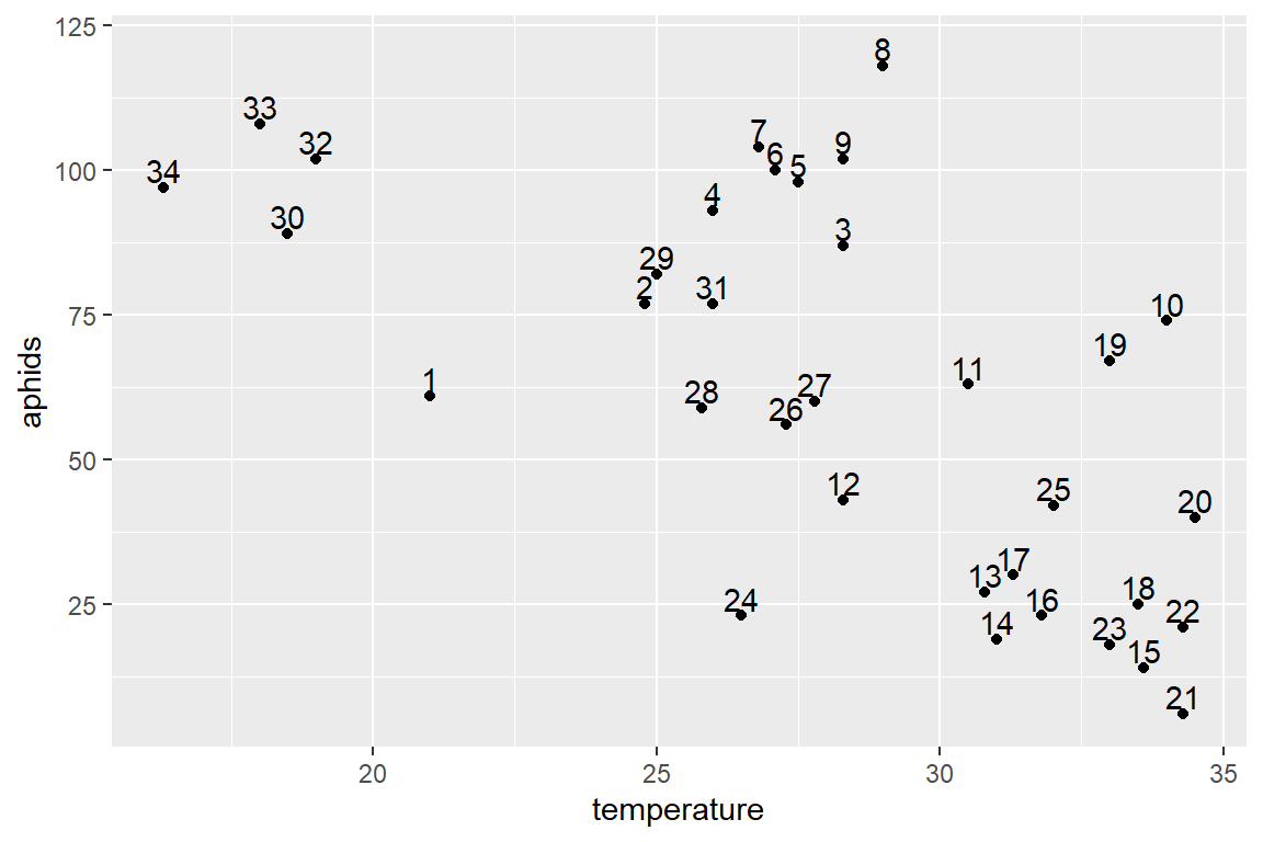
# Now let's consider RH and do the same thing
temp2 <- ggplot(aphids_data, aes(x=humidity, y=aphids, label=lot))
temp2 + geom_point() + geom_text(hjust=0.5, nudge_y=3) #Maybe a bit different grouping" 6-9, 33 and 34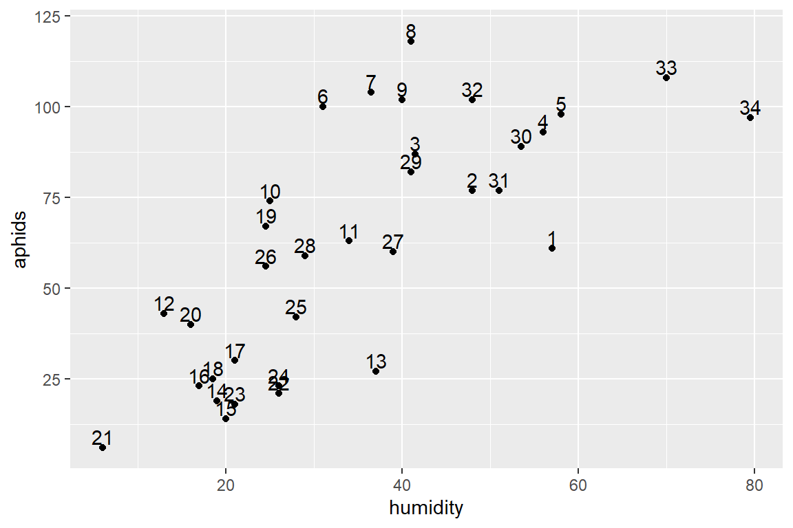
# In 3-dimensiones? This example comes from the package *scatterplot3d*

with(aphids_data, scatterplot3d(temperature, humidity, aphids, angle=75)) 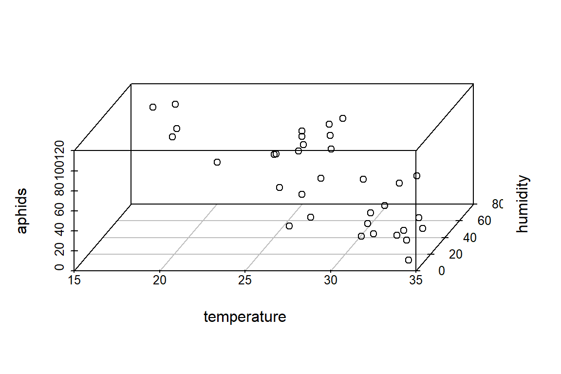
Multiple regression with interactions
Given that individually, we see different relationships between the number of aphids with temperature or relative humidity, we might want to consider if there is an interaction between those two factors that helps to explain the overall relationship.
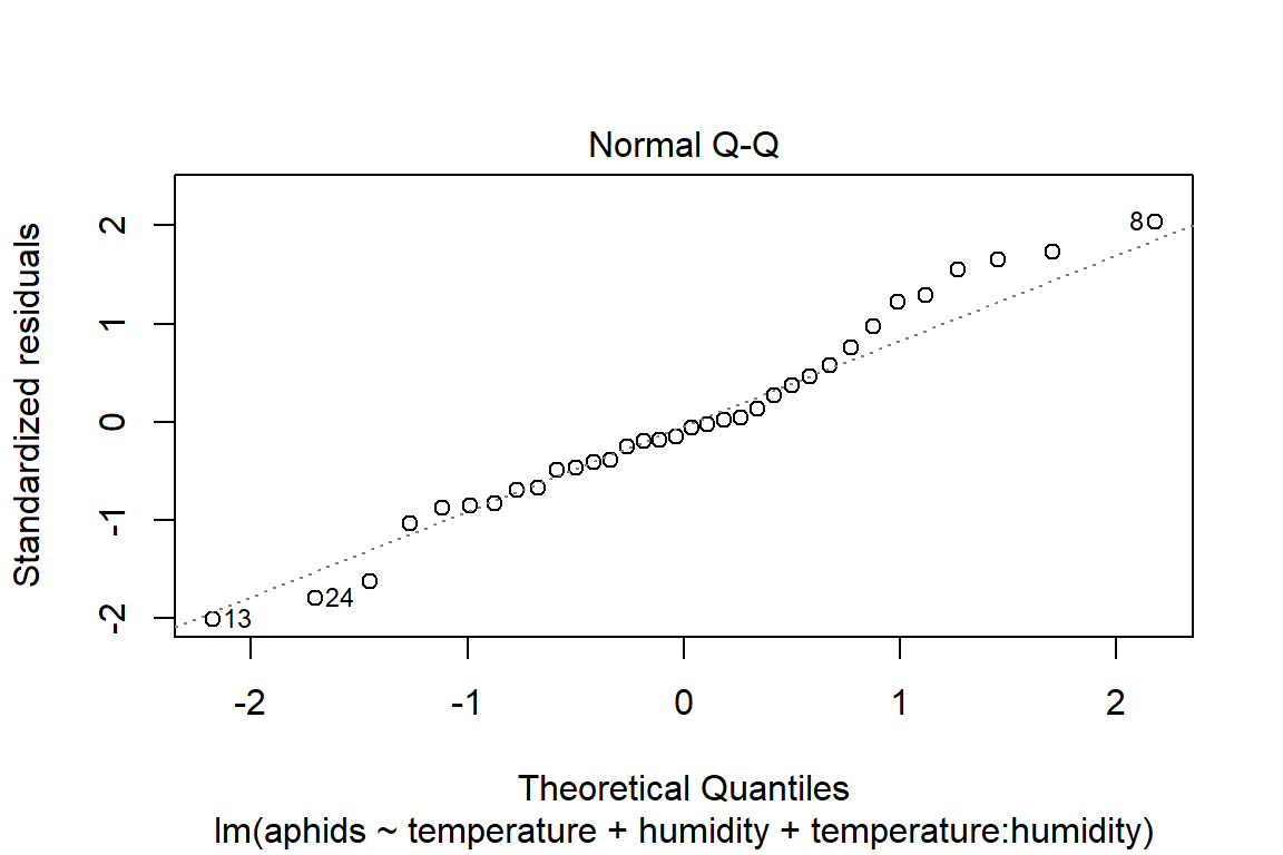
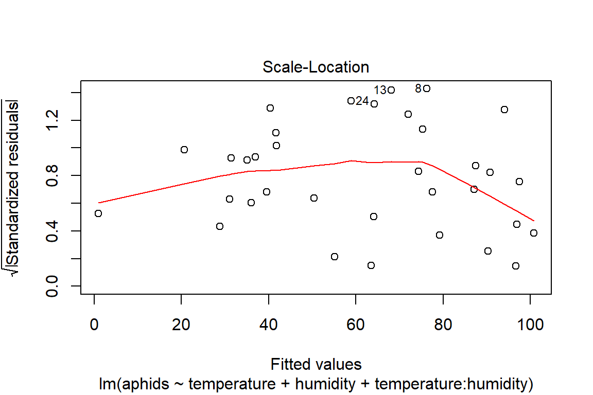
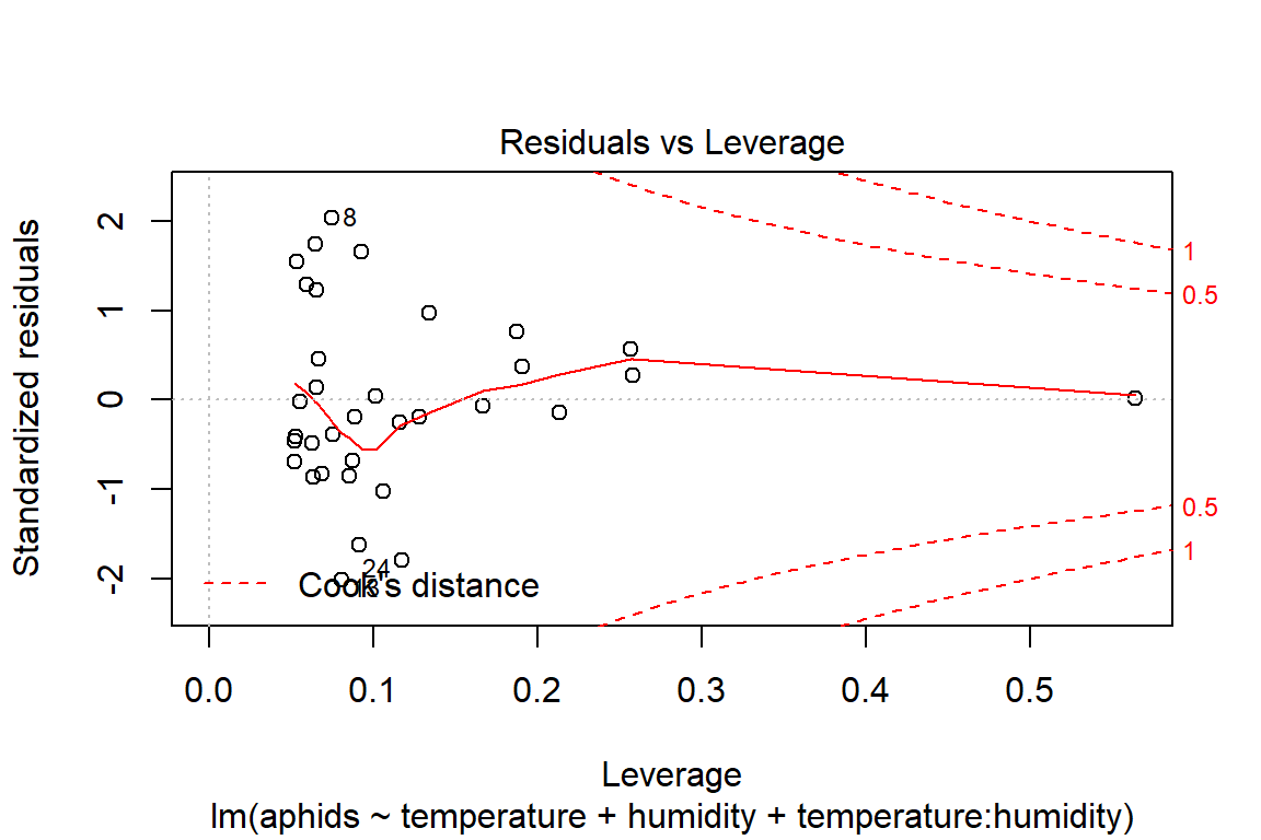
model4 <- with(aphids_data, lm(aphids ~ temperature + humidity + temperature:humidity))

anova(model4)
## Analysis of Variance Table
##
## Response: aphids
## Df Sum Sq Mean Sq F value Pr(>F)
## temperature 1 15194.8 15194.8 33.506 2.522e-06 ***
## humidity 1 4813.1 4813.1 10.613 0.002789 **
## temperature:humidity 1 2764.0 2764.0 6.095 0.019474 *
## Residuals 30 13604.8 453.5
## ---
## Signif. codes: 0 '***' 0.001 '**' 0.01 '*' 0.05 '.' 0.1 ' ' 1summary(model4) ##
## Call:
## lm(formula = aphids ~ temperature + humidity + temperature:humidity)
##
## Residuals:
## Min 1Q Median 3Q Max
## -41.13 -12.87 -2.02 10.25 41.75
##
## Coefficients:
## Estimate Std. Error t value Pr(>|t|)
## (Intercept) 150.70989 68.02395 2.216 0.0345 *
## temperature -4.72276 2.11121 -2.237 0.0329 *
## humidity -1.29670 1.11576 -1.162 0.2543
## temperature:humidity 0.09728 0.03940 2.469 0.0195 *
## ---
## Signif. codes: 0 '***' 0.001 '**' 0.01 '*' 0.05 '.' 0.1 ' ' 1
##
## Residual standard error: 21.3 on 30 degrees of freedom
## Multiple R-squared: 0.626, Adjusted R-squared: 0.5886
## F-statistic: 16.74 on 3 and 30 DF, p-value: 1.414e-06plot(model4)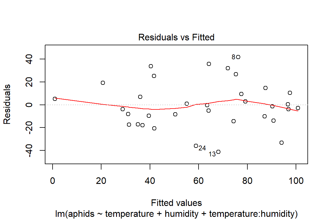
# Assumptions = values, model4
rstudent(model4)
## 1 2 3 4 5 6 7 8 9 10 11 12 13 14 15 16 17 18 19 20 21 22 23 24 25 26 27 28 29 30 31 32 33 34
## -1.67738460 -0.48588149 0.45590218 -0.19523576 -0.14531052 1.79972032 1.58449094 2.15886689 1.30727332 1.70840183 -0.02181518 0.36068272 -2.12994645 -0.86808331 -0.85354897 -0.38866846 -0.45693592 -0.18387477 1.23775270 0.97153371 0.27052672 -1.03205411 -0.82508336 -1.86536030 -0.40145315 0.04498291 -0.68446574 -0.24802524 0.13423194 -0.06323885 -0.67115336 0.75218833 0.56505021 0.02067808dfbetas(model4)## (Intercept) temperature humidity temperature:humidity
## 1 -0.0949334782 0.104709362 -0.039584196 0.019350004
## 2 -0.0434083991 0.051676363 0.047346765 -0.063039334
## 3 0.0104511179 -0.020483667 -0.043004153 0.068644149
## 4 0.0125973436 -0.003428996 0.005585795 -0.027700059
## 5 0.0200060874 -0.009982149 0.004443134 -0.028864368
## 6 0.3651795277 -0.341307478 -0.317703892 0.249350618
## 7 0.2422524883 -0.242541747 -0.242297450 0.232776103
## 8 -0.0109075193 -0.042140260 -0.177929199 0.320976539
## 9 0.0498830523 -0.072826504 -0.129655838 0.189283832
## 10 -0.3408072725 0.358785369 0.217261311 -0.151702669
## 11 0.0005263790 -0.000316099 0.001062068 -0.002009342
## 12 0.1221549093 -0.098424293 -0.075269257 0.020228157
## 13 0.1333989598 -0.088122021 0.090421220 -0.242562866
## 14 -0.0418864697 0.008011790 0.011031748 0.038058296
## 15 0.1317295973 -0.158260224 -0.117120422 0.123141864
## 16 0.0004605123 -0.017956896 -0.015762200 0.038604856
## 17 -0.0058300098 -0.008533870 -0.000619253 0.017463648
## 18 0.0260840050 -0.032918740 -0.025833607 0.029557943
## 19 -0.1563373872 0.174924757 0.097882894 -0.076671310
## 20 -0.2133463221 0.258866254 0.220017614 -0.243411245
## 21 -0.0520591385 0.077908687 0.084254567 -0.115605524
## 22 0.2314600667 -0.237322197 -0.139947666 0.086596590
## 23 0.0925507109 -0.115811898 -0.079585871 0.087209322
## 24 -0.5799971247 0.525151313 0.447129697 -0.289295996
## 25 0.0304683047 -0.032541539 -0.007414919 -0.003043043
## 26 0.0122044840 -0.010813140 -0.009331422 0.005713728
## 27 -0.0499259797 0.058126678 0.078027579 -0.098076089
## 28 -0.0786659661 0.072746679 0.061679949 -0.042751118
## 29 0.0246830038 -0.024958336 -0.021748326 0.020466850
## 30 -0.0135483304 0.012244012 0.001928902 0.002110430
## 31 -0.0027225130 0.024986567 0.044656549 -0.096290927
## 32 0.2502942582 -0.232060720 -0.113674644 0.047457190
## 33 -0.1102356148 0.113536109 0.212046646 -0.197252978
## 34 -0.0122551182 0.012733935 0.018960381 -0.017832210dffits(model4)## 1 2 3 4 5 6 7 8 9 10 11 12 13 14 15 16 17 18 19 20 21 22 23 24 25 26 27 28 29 30 31 32 33 34
## -0.531609206 -0.125502391 0.122090070 -0.074914358 -0.075725395 0.474770847 0.377244053 0.613987196 0.327877853 0.546849311 -0.005271111 0.175211526 -0.630865880 -0.225538194 -0.260429456 -0.111153445 -0.107334987 -0.057484681 0.327640435 0.381923652 0.159601123 -0.354887689 -0.224599512 -0.679748019 -0.094906727 0.015111134 -0.160394451 -0.089969303 0.035517257 -0.028285597 -0.207379175 0.361507505 0.332123809 0.023506774covratio(model4)## 1 2 3 4 5 6 7 8 9 10 11 12 13 14 15 16 17 18 19 20 21 22 23 24 25 26 27 28 29 30 31 32 33 34
## 0.8701623 1.1826549 1.1927973 1.3069641 1.4520128 0.8020052 0.8681666 0.6819798 0.9680977 0.8603410 1.2120133 1.3903653 0.6965068 1.1033099 1.1335691 1.2134151 1.1742397 1.2513168 0.9974108 1.1632187 1.5283511 1.1085842 1.1210624 0.8245063 1.1827248 1.2741137 1.1331044 1.2849849 1.2223690 1.3735892 1.1795590 1.3049070 1.4748564 2.6250656cooks.distance(model4)## 1 2 3 4 5 6 7 8 9 10 11 12 13 14 15 16 17 18 19 20 21 22 23 24 25 26 27 28 29 30 31 32 33 34
## 6.662438e-02 4.040602e-03 3.827564e-03 1.449516e-03 1.481939e-03 5.243821e-02 3.387265e-02 8.399563e-02 2.625550e-02 7.026714e-02 7.185558e-06 7.903960e-03 8.900520e-02 1.282220e-02 1.711070e-02 3.178723e-03 2.958219e-03 8.536139e-04 2.636942e-02 3.653477e-02 6.571137e-03 3.141810e-02 1.274688e-02 1.066957e-01 2.316596e-03 5.905097e-05 6.547598e-03 2.088968e-03 3.260411e-04 2.068874e-04 1.095216e-02 3.315175e-02 2.821681e-02 1.429035e-04# Graphically from olsrr package
ols_plot_resid_stud(model4)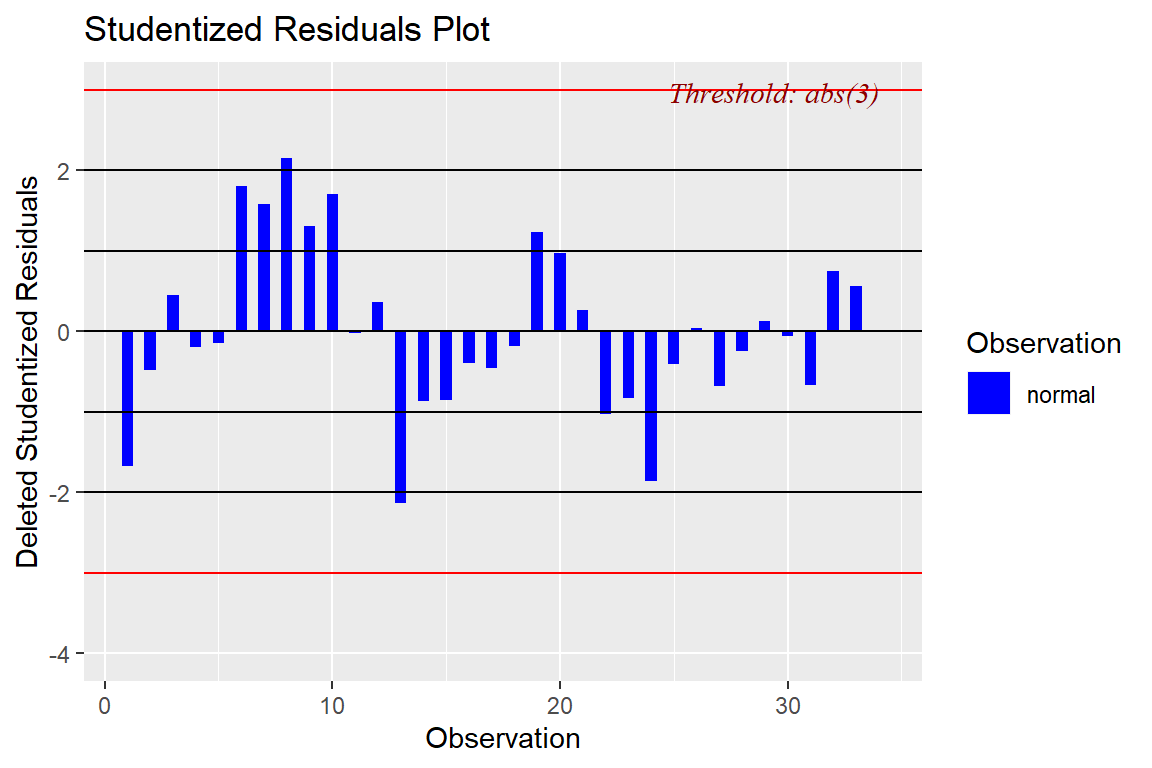
ols_plot_dfbetas(model4)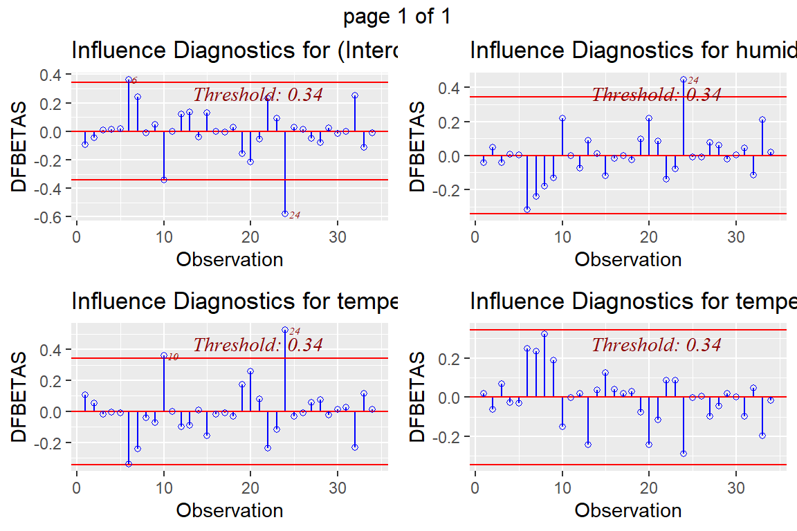
ols_plot_dffits(model4)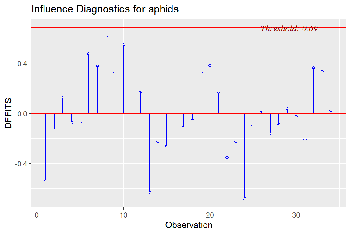
ols_plot_cooksd_chart(model4)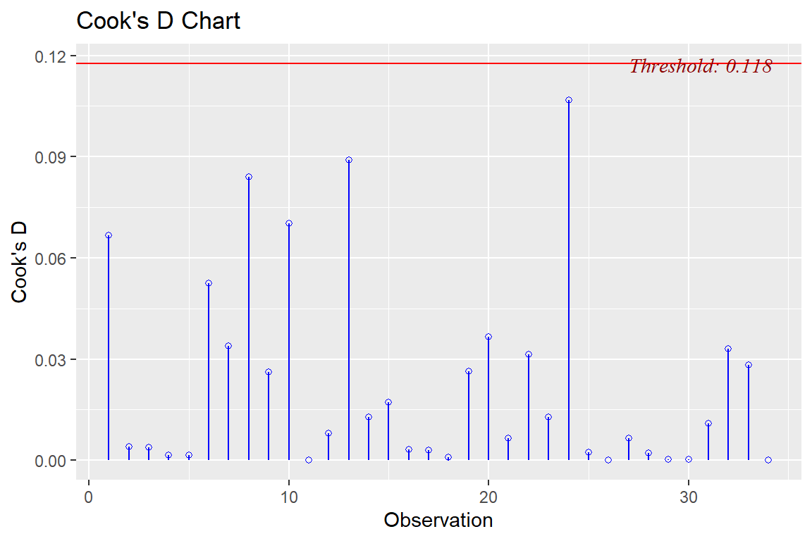
# Compare the different models
anova(model1, model3) # model 3 better
## Analysis of Variance Table
##
## Model 1: aphids ~ temperature
## Model 2: aphids ~ temperature + humidity
## Res.Df RSS Df Sum of Sq F Pr(>F)
## 1 32 21182
## 2 31 16369 1 4813.1 9.1151 0.005038 **
## ---
## Signif. codes: 0 '***' 0.001 '**' 0.01 '*' 0.05 '.' 0.1 ' ' 1anova(model2, model3) # model 2 mejor (only RH)## Analysis of Variance Table
##
## Model 1: aphids ~ humidity
## Model 2: aphids ~ temperature + humidity
## Res.Df RSS Df Sum of Sq F Pr(>F)
## 1 32 16486
## 2 31 16369 1 117.18 0.2219 0.6409anova(model2, model4) # the interaction improved the model?## Analysis of Variance Table
##
## Model 1: aphids ~ humidity
## Model 2: aphids ~ temperature + humidity + temperature:humidity
## Res.Df RSS Df Sum of Sq F Pr(>F)
## 1 32 16486
## 2 30 13605 2 2881.2 3.1767 0.05606 .
## ---
## Signif. codes: 0 '***' 0.001 '**' 0.01 '*' 0.05 '.' 0.1 ' ' 1anova(model3, model4) # the interaction improved the model## Analysis of Variance Table
##
## Model 1: aphids ~ temperature + humidity
## Model 2: aphids ~ temperature + humidity + temperature:humidity
## Res.Df RSS Df Sum of Sq F Pr(>F)
## 1 31 16369
## 2 30 13605 1 2764 6.095 0.01947 *
## ---
## Signif. codes: 0 '***' 0.001 '**' 0.01 '*' 0.05 '.' 0.1 ' ' 1# Remember that once we have a model selected, we should examine the assumptions in greater detailPredictions
To close our discussion, let’s again look at the function predict using model 4.
# Let's start by considering the average values for temperature and relative humidity
mean(temperature)
## [1] 28.08529mean(humidity)## [1] 35.19118observation <- data.frame(temperature=mean(temperature), humidity=mean(humidity))
predict(object=model4, newdata=observation, interval="confidence")## fit lwr upr
## 1 68.58645 59.30643 77.86646predict(object=model4, newdata=observation, interval="predict")## fit lwr upr
## 1 68.58645 24.11635 113.0565# Looking at all observations in the database
intervals<-predict(model4, interval="confidence")
intervals## fit lwr upr
## 1 94.0665692 80.927158 107.20598
## 2 87.1482874 76.271599 98.02498
## 3 77.4955105 66.245093 88.74593
## 4 96.9454425 81.365016 112.52587
## 5 100.7900752 80.691122 120.88903
## 6 64.2519748 53.158443 75.34551
## 7 71.9715847 61.898562 82.04461
## 8 76.2533767 64.356209 88.15054
## 9 75.3109441 64.730640 85.89125
## 10 40.4082060 27.149656 53.66676
## 11 63.4592842 53.244672 73.67390
## 12 35.9887485 16.985340 54.99216
## 13 68.1334763 55.782306 80.48465
## 14 36.9661205 26.029726 47.90252
## 15 31.4646380 18.772561 44.15671
## 16 31.0728691 19.114485 43.03125
## 17 39.6002445 29.654831 49.54566
## 18 28.7989865 15.821797 41.77618
## 19 41.7421198 30.613084 52.87116
## 20 20.7271297 4.815514 36.63875
## 21 0.9596999 -21.139235 23.05864
## 22 41.7610595 27.618756 55.90336
## 23 35.0445138 23.621299 46.46773
## 24 58.8698369 43.979310 73.76036
## 25 50.4385954 40.432771 60.44442
## 26 55.0764466 41.227039 68.92585
## 27 74.3189517 64.396268 84.24164
## 28 64.0447598 49.214277 78.87524
## 29 79.1902050 68.065480 90.31493
## 30 90.2502594 72.492852 108.00767
## 31 90.7822943 77.942971 103.62162
## 32 87.4570502 68.617765 106.29634
## 33 97.5065531 75.468470 119.54464
## 34 96.7041862 64.049441 129.35893predictions<-predict(model4, interval="predict")## Warning in predict.lm(model4, interval = "predict"): predictions on current data refer to _future_ responsespredictions## fit lwr upr
## 1 94.0665692 48.634034 139.49910
## 2 87.1482874 42.317791 131.97878
## 3 77.4955105 32.572877 122.41814
## 4 96.9454425 50.747815 143.14307
## 5 100.7900752 52.879335 148.70082
## 6 64.2519748 19.368375 109.13557
## 7 71.9715847 27.329263 116.61391
## 8 76.2533767 31.164423 121.34233
## 9 75.3109441 30.551432 120.07046
## 10 40.4082060 -5.058928 85.87534
## 11 63.4592842 18.784802 108.13377
## 12 35.9887485 -11.472822 83.45032
## 13 68.1334763 22.922609 113.34434
## 14 36.9661205 -7.878900 81.81114
## 15 31.4646380 -13.840548 76.76982
## 16 31.0728691 -14.032275 76.17801
## 17 39.6002445 -5.013457 84.21395
## 18 28.7989865 -16.586898 74.18487
## 19 41.7421198 -3.150269 86.63451
## 20 20.7271297 -25.583243 67.03750
## 21 0.9596999 -47.823843 49.74324
## 22 41.7610595 -3.971597 87.49372
## 23 35.0445138 -9.921706 80.01073
## 24 58.8698369 12.900294 104.83938
## 25 50.4385954 5.811388 95.06580
## 26 55.0764466 9.433515 100.71938
## 27 74.3189517 29.710312 118.92759
## 28 64.0447598 18.094631 109.99489
## 29 79.1902050 34.298885 124.08152
## 30 90.2502594 43.273705 137.22681
## 31 90.7822943 45.435637 136.12895
## 32 87.4570502 40.060956 134.85314
## 33 97.5065531 48.750546 146.26256
## 34 96.7041862 42.318494 151.08988Summary
The objective in this exercise was to introduce the concept of using multiple regression to build a model. This provides a base also as you move forward in your modeling work to think about things like hidden interactions, which is often very common in complex datasets and can often drive aspects of things like machine learning.