Background
Nonlinear regression is an important modeling tool for looking at more compliated biological, physiological, etc., relationships. This introductory exercise describes some of the concepts that one should consider when analyzing nonlinear data. The process is iterative for modeling fitting, meaning that the parameters are estimated in a stepwise fashion. In Plant Pathology this is a useful tool for things like disease development over time. These models can be further extended to incorporated additional factors like treatments, years, among other things, to study the overall behavior and observed variability.
# Note that for this example, we will keep the tools to those that are available in the base package

library(tidyverse)
Data
This work originated in Costa Rica and focused on growth and development of onion in the northern areas of the Province of Cartago. Growth was measured using whole plant biomass. The goal was to understand how different varieties performed in this zone and future work would examine the impact of different management tactics and pests on improving overall productivity.
The data strcuture for the orginal worked involved three cultivars but for the exercise we will only focus on one of those, which is called Alvara.
- dap = days after planting
- gdd = growing degree days based on threshold temperatures for onion
- root = root dry weight (grams)
- buld = bulb dry weight (grams)
- aerial = aerial biomass dry weight (grams)
- total = total dry weight considering the above measurements
dap <- c(11, 18, 26, 33, 40, 47, 56, 61, 69, 82, 96, 111, 124)
gdd <- c(148, 233, 327, 410, 492, 575, 686, 746, 837, 993, 1158, 1335, 1484)
root <- c(0.04, 0.019, 0.113, 0.044, 0.045, 0.056, 0.08, 0.114, 0.109, 0.116, 0.098, 0.101, 0.066)
bulb <- c(0.137, 0.166, 0.289, 0.2, 0.292, 0.298, 0.474, 0.416, 1.236, 2.594, 6.265, 6.174,
22.521)
aerial <- c(0.162, 0.191, 0.308, 0.243, 0.25, 0.343, 0.988, 0.962, 2.593, 3.379, 2.83, 5.054,
2.748)
total <- c(0.34, 0.376, 0.711, 0.487, 0.587, 0.698, 1.542, 1.492, 3.938, 6.089, 9.193, 11.329,
25.334)

alvara <- data.frame(dap, gdd, root, bulb, aerial, total)
Graphical representation - preliminary
Graphically, we will use some basic tools to look at the overall behavior.
## The predictive factor is growing degree days, assuming that best explains the overall growth and development

with(alvara, plot(x=gdd, y=root, type="b", lty=1, lwd=2, pch=19, col="black"))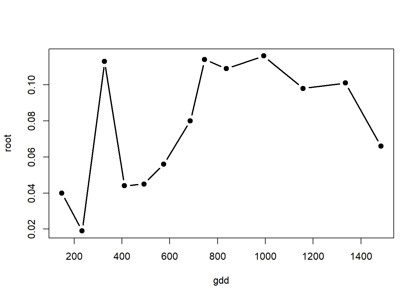
with(alvara, plot(x=gdd, y=bulb, type="b", lty=1, lwd=2, pch=19, col="black"))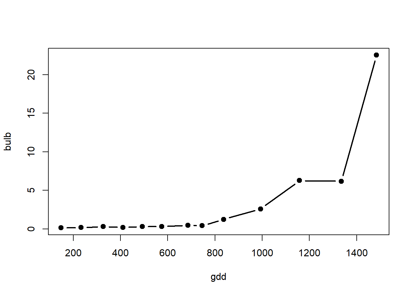
with(alvara, plot(x=gdd, y=aerial, type="b", lty=1, lwd=2, pch=19, col="black"))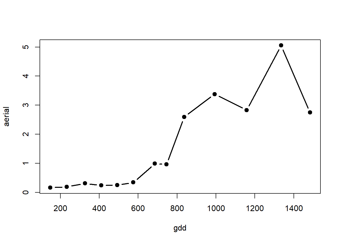
with(alvara, plot(x=gdd, y=total, type="b", lty=1, lwd=2, pch=19, col="black"))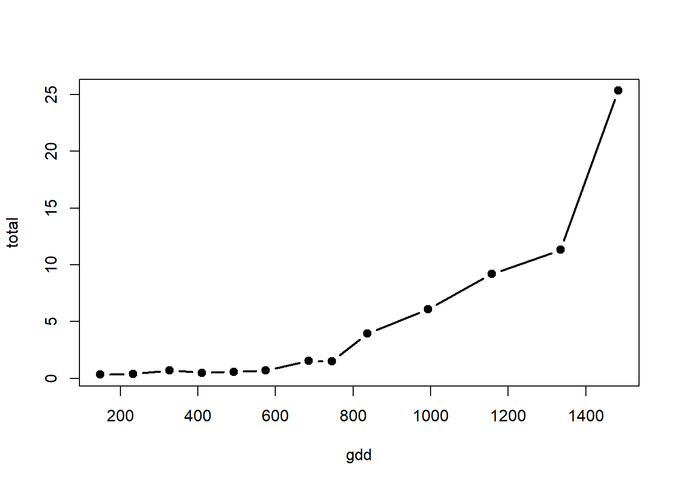
Modeling
Selecting a nonlinear model depends on many factors especially taking into account the biological relationship. In preliminary analyses with data of this type for onion, we saw two possible nonlinear models that best describe the relationships. In the first case the development was bell-shaped, showing increases until a specific point in the developmental process when dry weight was reduced. The second curve tupe was exponential and related to the ultimate growth phases just prior to harvest. Even though growth is not infinite, we still recognize that this model may explain well the relationship and is interpretable.
Model 1.
\[ DW = \alpha * exp(-\beta * (gdd-\gamma)^2)\]
Where, DW is the dry weight (g), \(\alpha\) is the measure of initial dry weight the start of evaluations (0 gdds), \(\beta\) is the growth rate, and \(\gamma\) represents the inflexion point in the process. “gdd” are the accumulated growing degree days.
Model 2.
\[ DW = X_0 * exp (K * gdd) \]
where, DW is the dry weight (g), \(X_0\) is the condition where there has been no accumulation of heat units, and K is the growth rate as a function of the accumulated growing degree days (gdd).
In both cases, it is important to take into account that the model will be adjusted based on the definition of the initial starting parameters. There are different methods to define initial starting parameters, including:
- using a grid search approach to find the best combination of all parameters in the model
- using preliminary analyses to define the parameters (can be based on similar data to your situation)
- functional estimate based on the model form and your knowledge about the system
- genetic algorithms, see for example, https://en.wikipedia.org/wiki/Genetic_algorithm
- in R there are also for some of the models there are functions that will obtain initial starting parameters (see: http://www.apsnet.org/edcenter/advanced/topics/EcologyAndEpidemiologyInR/DiseaseProgress/Pages/NonlinearRegression.aspx)
For the following examples, we will use the third method based on knowledge of the crop physiology and preliminary analyses.
Model 1
## Variable = root dry weight
## nls = nonlinear least squares
## start=list() provides the input to define the initial starting values for the parameters

regnl1 <- nls(root ~ alpha * exp(-beta*(gdd-gamma)^2),
              start=list(alpha = 0.15, beta = 0.0000002, gamma = 900), trace=TRUE, data=alvara)
## 0.07027501 : 1.5e-01 2.0e-07 9.0e+02
## 0.008673095 : 1.007217e-01 7.854471e-07 1.308727e+03
## 0.007106798 : 9.761952e-02 1.203522e-06 1.002286e+03
## 0.006594237 : 1.069288e-01 1.562084e-06 1.021834e+03
## 0.006588507 : 1.079002e-01 1.618805e-06 1.016275e+03
## 0.006588451 : 1.079549e-01 1.621248e-06 1.016766e+03
## 0.00658845 : 1.079619e-01 1.621827e-06 1.016741e+03
## 0.00658845 : 1.079626e-01 1.621871e-06 1.016743e+03summary(regnl1)##
## Formula: root ~ alpha * exp(-beta * (gdd - gamma)^2)
##
## Parameters:
## Estimate Std. Error t value Pr(>|t|)
## alpha 1.080e-01 1.268e-02 8.516 6.78e-06 ***
## beta 1.622e-06 7.130e-07 2.275 0.0462 *
## gamma 1.017e+03 9.913e+01 10.257 1.26e-06 ***
## ---
## Signif. codes: 0 '***' 0.001 '**' 0.01 '*' 0.05 '.' 0.1 ' ' 1
##
## Residual standard error: 0.02567 on 10 degrees of freedom
##
## Number of iterations to convergence: 7
## Achieved convergence tolerance: 2.89e-06## Predictions
regnl_pred <- predict(regnl1, data.frame(gdd=seq(100,1500,25)))
## Database of predictions over a range of gdds
predictions <- data.frame(gdd=seq(100,1500,25), pred=regnl_pred)
## Graphically
ej1 <- ggplot()
ej1 +
geom_point(data=alvara, aes(x=gdd, y=root)) +
geom_line(data=predictions, aes(x=gdd, y=pred), lty=1, lwd=1.5)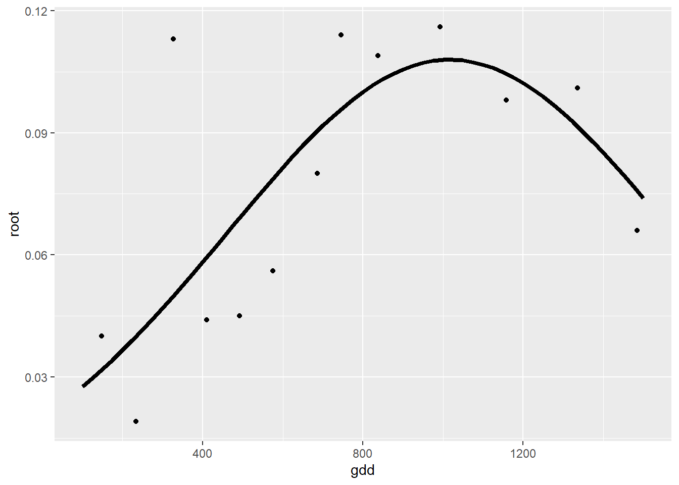
Model 2
## Variable = total dry weight

regnl2 <- nls(total ~ x0 * exp(k * gdd), start = list(x0=0.5, k=0.0002), trace=TRUE, data=alvara)
## 838.571 : 5e-01 2e-04
## 745.1133 : 0.164848298 0.001679615
## 547.7136 : 0.066722470 0.002956091
## 231.1729 : 0.086874301 0.003337606
## 66.82676 : 0.124641432 0.003367594
## 17.75713 : 0.161921536 0.003372197
## 17.75511 : 0.16183068 0.00337153
## 17.75511 : 0.16184411 0.00337147summary(regnl2)##
## Formula: total ~ x0 * exp(k * gdd)
##
## Parameters:
## Estimate Std. Error t value Pr(>|t|)
## x0 0.1618441 0.0645079 2.509 0.029 *
## k 0.0033715 0.0002832 11.905 1.26e-07 ***
## ---
## Signif. codes: 0 '***' 0.001 '**' 0.01 '*' 0.05 '.' 0.1 ' ' 1
##
## Residual standard error: 1.27 on 11 degrees of freedom
##
## Number of iterations to convergence: 7
## Achieved convergence tolerance: 5.642e-06## Predictions
regn2_pred <- predict(regnl2, data.frame(gdd=seq(100,1500,25)))
## Database of predictions
predictions <- data.frame(gdd=seq(100,1500,25), pred=regn2_pred)
## Graphically
ej2 <- ggplot()
ej2 +
geom_point(data=alvara, aes(x=gdd, y=total)) +
geom_line(data=predictions, aes(x=gdd, y=pred), lty=1, lwd=1.5)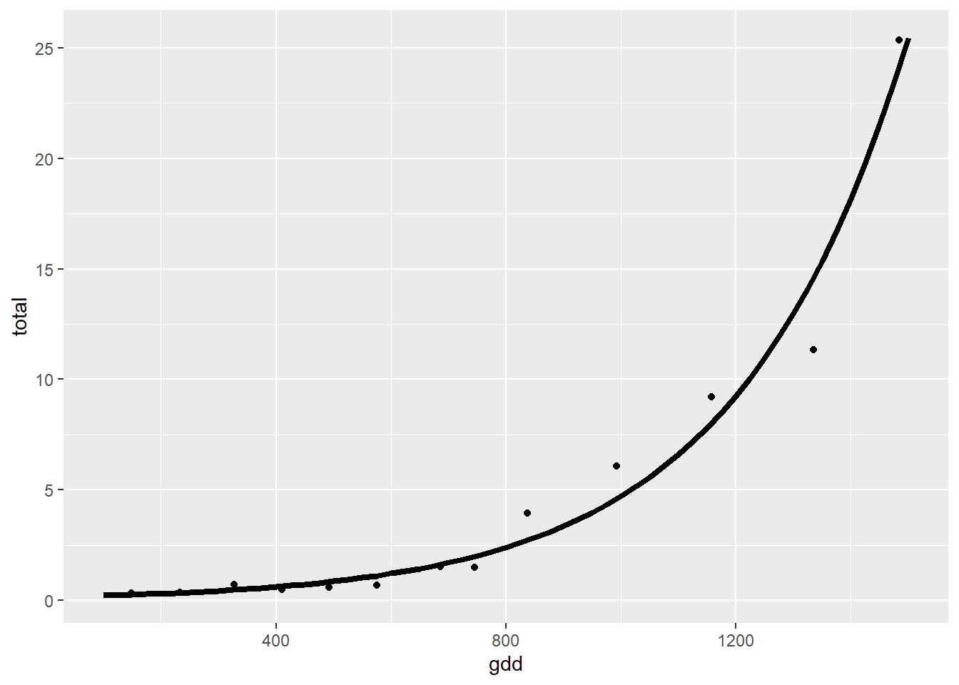
Exercises
Perform the same set of the analyses for the following measurements and initial parameter conditions:
Aerial dry weight, you can consider the following starting parameter values: start=list(alpha = 5, beta = 0.00002, gamma = 1100).
Bulb dry weight, you can consider the following starting parameter values: start=list(x0 = 0.5, k = 0.0002).