Background
In many studies, for example if one looks the relationship between nitrogen and yield for many cereal crops, the relationship is not linear, rather there is often a plateau where after a specific amount, the response decreases. A simpler linear-type model will explain some of the variability, but not very well. In these situations we can consider a polynomial form to the model.
We can define this relationship in general terms as the the relation betweeen the independent variable, \(x\), and the expected response, \(E(y|x)\).
Note: Very important with this type of analysis is to understand the software that you are using since often we focus on use \(X\) and \(X^2\), which depending on how those variables are defined, leads to high collinearity. This example illustrates that concept and provides methods to overcome the issue.
library(tidyverse)
library(Hmisc)
library(corrplot)
library(readr)
library(HH)
library(car)
Data
For this example, we have the following situation:
- Density = Seeding density (number of plants per \(m^2\))
- Yield = quantity of biomass
density <- rep(c(10,20,30,40,50), each=3)
yield <- c(12.2, 11.4, 12.4, 16, 15.5, 16.5, 18.6, 20.2, 18.2, 17.6, 19.3, 17.1, 18, 16.4, 16.6)

densities <- data.frame(density, yield)
Linear regression
To start, we will build a simple linear regression models and examine the overall model fit, including model assumptions.
model1 <- lm(yield~density)
anova(model1)
## Analysis of Variance Table
##
## Response: yield
## Df Sum Sq Mean Sq F value Pr(>F)
## density 1 43.20 43.200 10.825 0.005858 **
## Residuals 13 51.88 3.991
## ---
## Signif. codes: 0 '***' 0.001 '**' 0.01 '*' 0.05 '.' 0.1 ' ' 1summary(model1)##
## Call:
## lm(formula = yield ~ density)
##
## Residuals:
## Min 1Q Median 3Q Max
## -2.6 -1.7 0.0 1.5 3.8
##
## Coefficients:
## Estimate Std. Error t value Pr(>|t|)
## (Intercept) 12.80000 1.20966 10.58 9.3e-08 ***
## density 0.12000 0.03647 3.29 0.00586 **
## ---
## Signif. codes: 0 '***' 0.001 '**' 0.01 '*' 0.05 '.' 0.1 ' ' 1
##
## Residual standard error: 1.998 on 13 degrees of freedom
## Multiple R-squared: 0.4544, Adjusted R-squared: 0.4124
## F-statistic: 10.82 on 1 and 13 DF, p-value: 0.005858plot(model1) # You hopefully can see that the model fit is not very good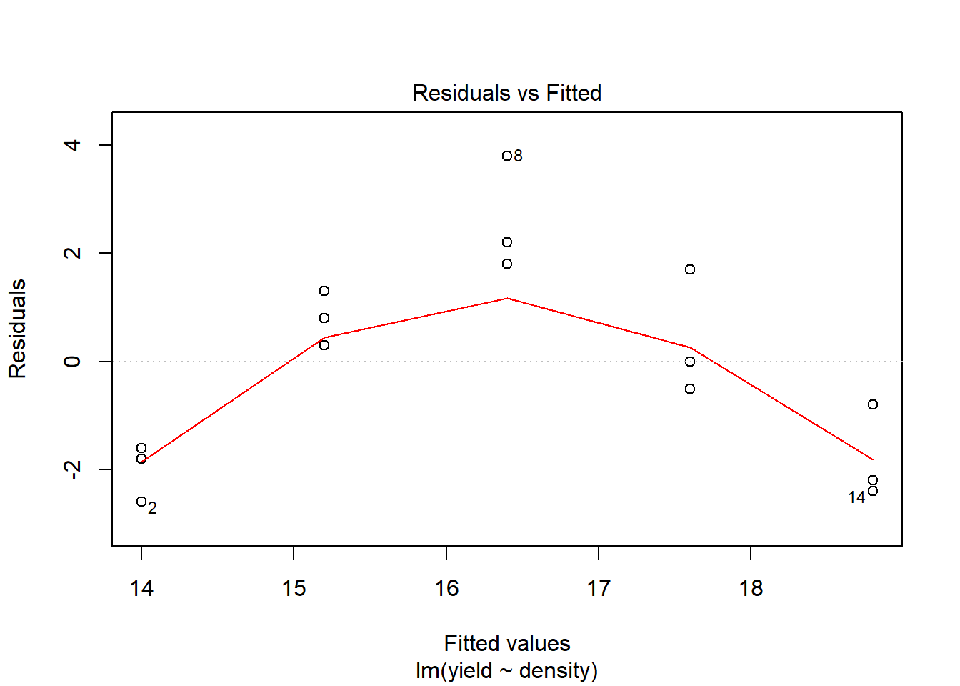
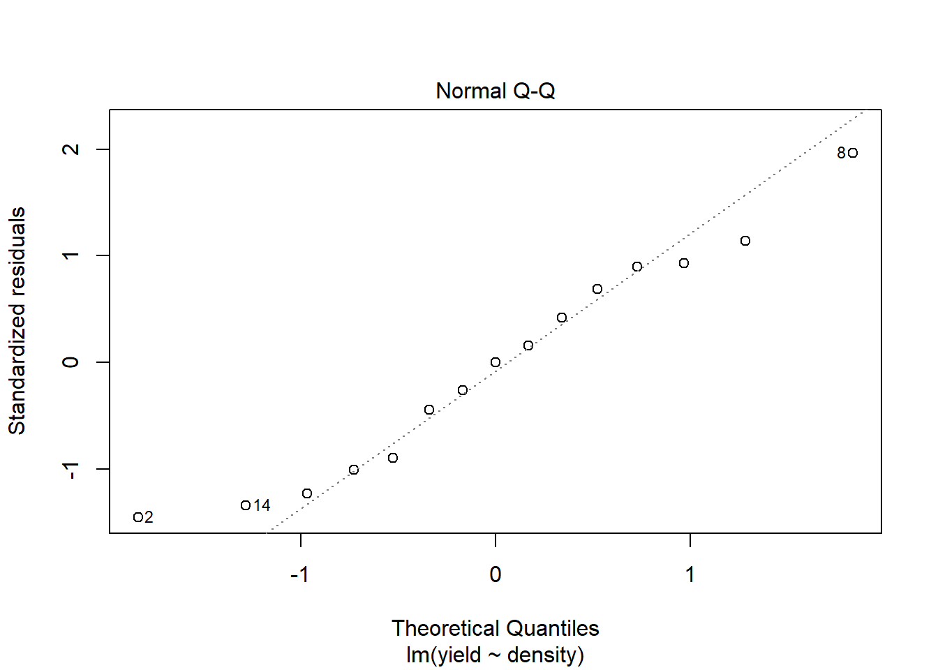
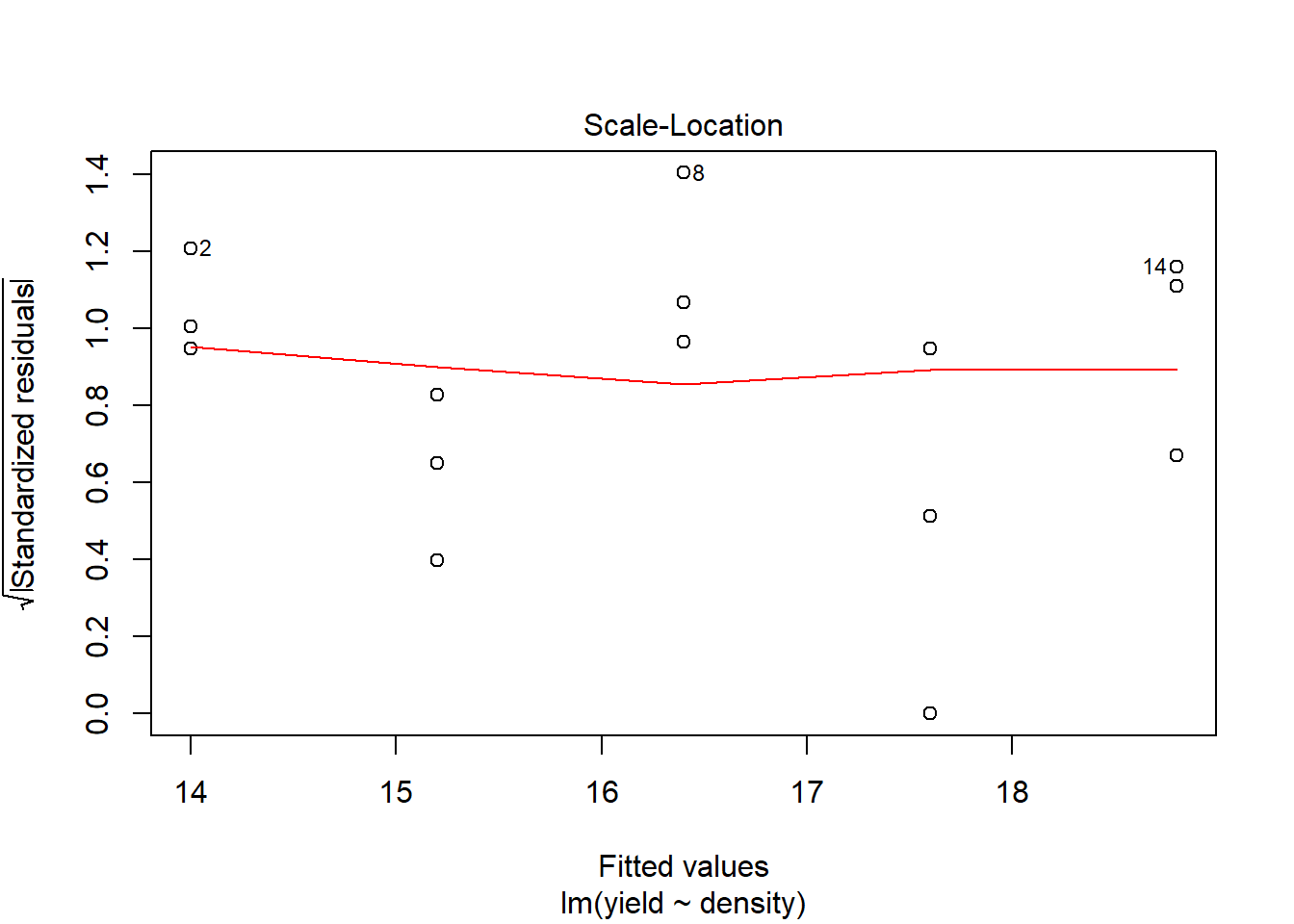
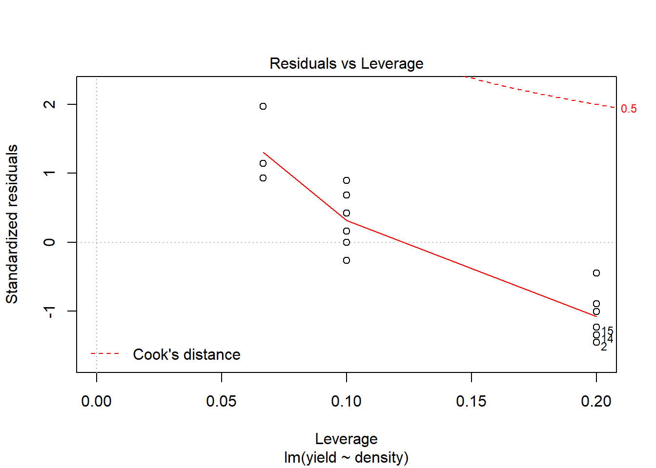
ci.plot(model1) # It should be obvious that the regression line does not reflect the actual relationship well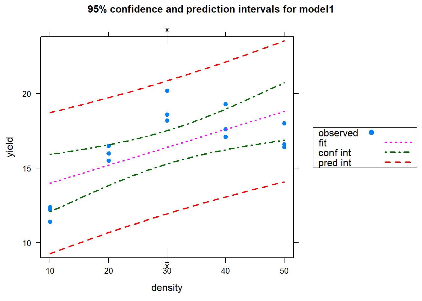
Quadratic regression 1
Given the result just seem with the simple linear regression, we will construct a quadratic model. The structure of the analysis is the same, but we will create a variable for density to reflect the squared term, \(density^2\).
# Define the density as a squared term (there are multiple ways to do this, but we will use a simple approach for now)

density2<-density^2

model2<-lm(yield~density + density2)

# Significance
anova(model2)
## Analysis of Variance Table
##
## Response: yield
## Df Sum Sq Mean Sq F value Pr(>F)
## density 1 43.20 43.200 52.470 1.024e-05 ***
## density2 1 42.00 42.000 51.012 1.177e-05 ***
## Residuals 12 9.88 0.823
## ---
## Signif. codes: 0 '***' 0.001 '**' 0.01 '*' 0.05 '.' 0.1 ' ' 1summary(model2)##
## Call:
## lm(formula = yield ~ density + density2)
##
## Residuals:
## Min 1Q Median 3Q Max
## -1.50 -0.50 -0.20 0.35 1.80
##
## Coefficients:
## Estimate Std. Error t value Pr(>|t|)
## (Intercept) 5.80000 1.12359 5.162 0.000236 ***
## density 0.72000 0.08563 8.409 2.25e-06 ***
## density2 -0.01000 0.00140 -7.142 1.18e-05 ***
## ---
## Signif. codes: 0 '***' 0.001 '**' 0.01 '*' 0.05 '.' 0.1 ' ' 1
##
## Residual standard error: 0.9074 on 12 degrees of freedom
## Multiple R-squared: 0.8961, Adjusted R-squared: 0.8788
## F-statistic: 51.74 on 2 and 12 DF, p-value: 1.259e-06# Assumptions
plot(model2)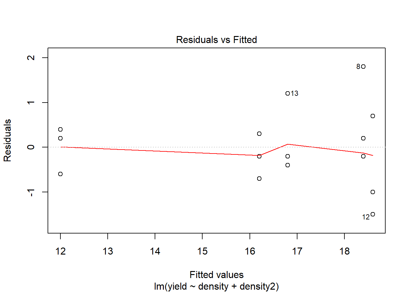
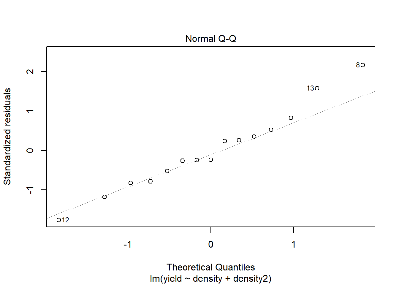
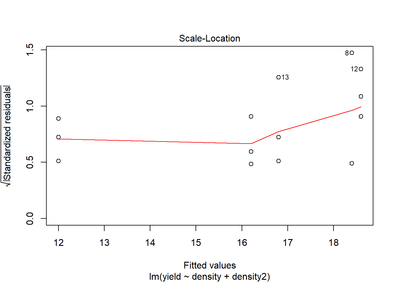
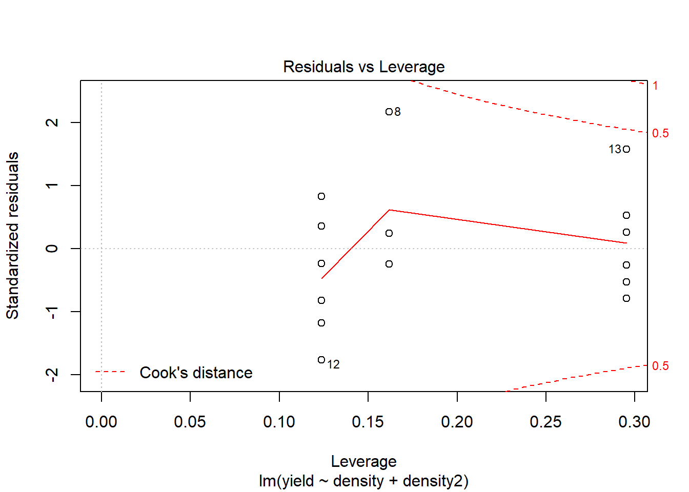
# Let's focus on comparing the two models based on Cook's Distance.
plot(model1, which=4) 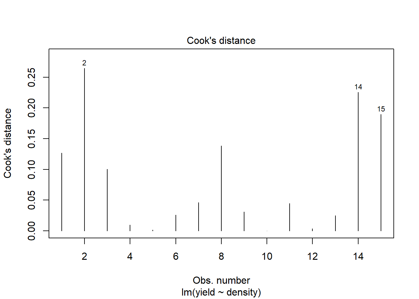
plot(model2, which=4) 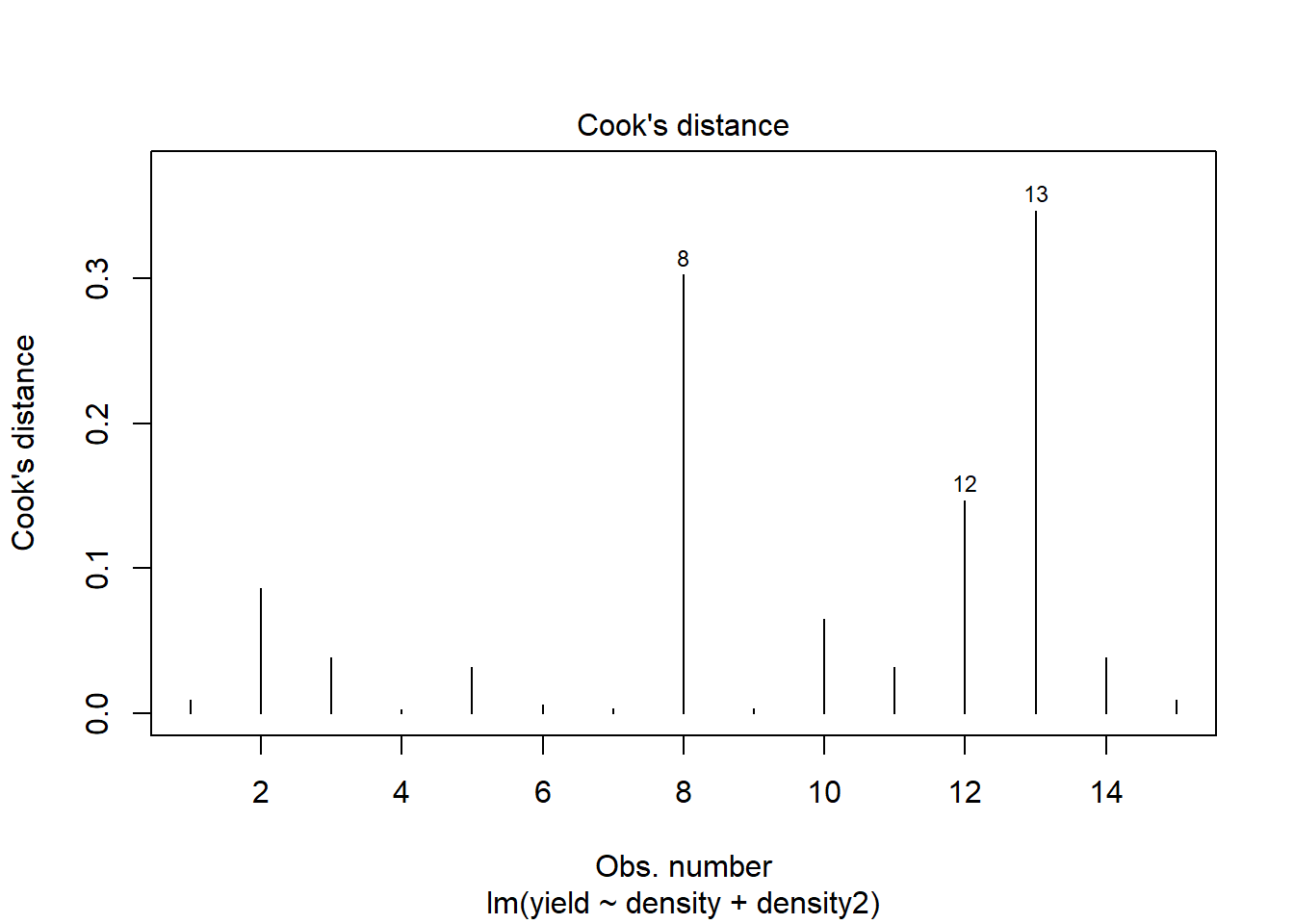
# F-test between model 1 and model 2
anova(model1, model2)
## Analysis of Variance Table
##
## Model 1: yield ~ density
## Model 2: yield ~ density + density2
## Res.Df RSS Df Sum of Sq F Pr(>F)
## 1 13 51.88
## 2 12 9.88 1 42 51.012 1.177e-05 ***
## ---
## Signif. codes: 0 '***' 0.001 '**' 0.01 '*' 0.05 '.' 0.1 ' ' 1# Additional tools to understand the model fit and model assumptions for the quadratic form
influence.measures(model2) # this is a general function to create the base for subsequent measurments## Influence measures of
## lm(formula = yield ~ density + density2) :
##
## dfb.1_ dfb.dnst dfb.dns2 dffit cov.r cook.d hat inf
## 1 1.46e-01 -0.1121 0.0927 0.1632 1.811 0.00963 0.295 *
## 2 -4.47e-01 0.3445 -0.2847 -0.5012 1.571 0.08663 0.295
## 3 2.94e-01 -0.2262 0.1870 0.3292 1.718 0.03850 0.295
## 4 3.67e-17 -0.0280 0.0373 -0.0849 1.461 0.00261 0.124
## 5 5.03e-17 -0.1007 0.1339 -0.3054 1.244 0.03199 0.124
## 6 -3.68e-17 0.0422 -0.0560 0.1278 1.436 0.00588 0.124
## 7 -5.44e-02 0.0764 -0.0779 0.1016 1.527 0.00373 0.162
## 8 -6.26e-01 0.8795 -0.8964 1.1687 0.349 0.30236 0.162
## 9 5.44e-02 -0.0764 0.0779 -0.1016 1.527 0.00373 0.162
## 10 2.07e-01 -0.2391 0.1976 -0.4506 1.025 0.06529 0.124
## 11 -1.40e-01 0.1620 -0.1339 0.3054 1.244 0.03199 0.124
## 12 3.39e-01 -0.3920 0.3240 -0.7388 0.601 0.14691 0.124
## 13 3.26e-01 -0.4683 0.6225 1.0961 0.919 0.34654 0.295
## 14 -9.79e-02 0.1406 -0.1870 -0.3292 1.718 0.03850 0.295
## 15 -4.85e-02 0.0697 -0.0927 -0.1632 1.811 0.00963 0.295 *dffits(model2)## 1 2 3 4 5 6
## 0.16317088 -0.50123382 0.32920738 -0.08494387 -0.30538465 0.12778710
## 7 8 9 10 11 12
## 0.10156307 1.16874641 -0.10156307 -0.45055886 0.30538465 -0.73883264
## 13 14 15
## 1.09610758 -0.32920738 -0.16317088dfbeta(model2)## (Intercept) density density2
## 1 1.702703e-01 -0.010000000 1.351351e-04
## 2 -5.108108e-01 0.030000000 -4.054054e-04
## 3 3.405405e-01 -0.020000000 2.702703e-04
## 4 4.299875e-17 -0.002500000 5.434783e-05
## 5 5.733167e-17 -0.008750000 1.902174e-04
## 6 -4.299875e-17 0.003750000 -8.152174e-05
## 7 -6.363636e-02 0.006818182 -1.136364e-04
## 8 -5.727273e-01 0.061363636 -1.022727e-03
## 9 6.363636e-02 -0.006818182 1.136364e-04
## 10 2.282609e-01 -0.020108696 2.717391e-04
## 11 -1.597826e-01 0.014076087 -1.902174e-04
## 12 3.423913e-01 -0.030163043 4.076087e-04
## 13 3.405405e-01 -0.037297297 8.108108e-04
## 14 -1.135135e-01 0.012432432 -2.702703e-04
## 15 -5.675676e-02 0.006216216 -1.351351e-04covratio(model2)## 1 2 3 4 5 6 7
## 1.8105775 1.5709359 1.7180496 1.4612786 1.2440860 1.4359881 1.5267335
## 8 9 10 11 12 13 14
## 0.3493908 1.5267335 1.0252651 1.2440860 0.6006431 0.9193090 1.7180496
## 15
## 1.8105775cooks.distance(model2)## 1 2 3 4 5 6
## 0.009626105 0.086634944 0.038504420 0.002611680 0.031993085 0.005876281
## 7 8 9 10 11 12
## 0.003732810 0.302357630 0.003732810 0.065292011 0.031993085 0.146907024
## 13 14 15
## 0.346539778 0.038504420 0.009626105vif(model2) # 26.71 is the value, values greater than 10 typically indicate high collinearity## density density2
## 26.71429 26.71429Quadratic regression 2
Given the result for the first quadratic regression that indicated high collinearity for \(density\) and \(density^2\), what we can do to remove this without affecting the analysis is to center the density variable and then run the analysis again. This is a very common practice to reduce the impact of not only high collinearity but also for cases for things like multivariate statistics where the scale for individual response variables can have high leverage on the overall analysis. The fuction, scale, allows us to the scale the density considering the mean value (we are not taking into account the variance, which is another common approach = location-scale type centering).
# Center and standardize the density variable

# This approach substracts the mean, scale=FALSE tells R that we do not take into account the standard deviation in the analysis
den_centered<-scale(density, center=TRUE, scale=FALSE)

# The same if we did this by "hand"
density-mean(density)
## [1] -20 -20 -20 -10 -10 -10 0 0 0 10 10 10 20 20 20# Create a new variable for density^2 based on centered values
den_centered2 <- den_centered^2
plot(den_centered, den_centered2)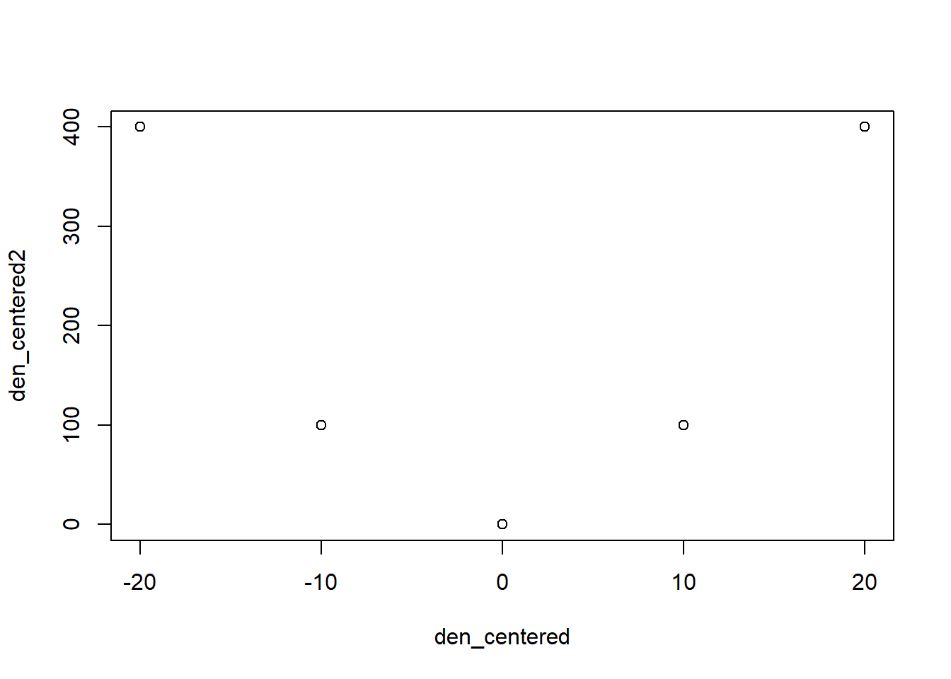
# Regression model with centered data

model3<-lm(yield~den_centered+den_centered2)
anova(model3)
## Analysis of Variance Table
##
## Response: yield
## Df Sum Sq Mean Sq F value Pr(>F)
## den_centered 1 43.20 43.200 52.470 1.024e-05 ***
## den_centered2 1 42.00 42.000 51.012 1.177e-05 ***
## Residuals 12 9.88 0.823
## ---
## Signif. codes: 0 '***' 0.001 '**' 0.01 '*' 0.05 '.' 0.1 ' ' 1summary(model3)##
## Call:
## lm(formula = yield ~ den_centered + den_centered2)
##
## Residuals:
## Min 1Q Median 3Q Max
## -1.50 -0.50 -0.20 0.35 1.80
##
## Coefficients:
## Estimate Std. Error t value Pr(>|t|)
## (Intercept) 18.40000 0.36511 50.396 2.44e-15 ***
## den_centered 0.12000 0.01657 7.244 1.02e-05 ***
## den_centered2 -0.01000 0.00140 -7.142 1.18e-05 ***
## ---
## Signif. codes: 0 '***' 0.001 '**' 0.01 '*' 0.05 '.' 0.1 ' ' 1
##
## Residual standard error: 0.9074 on 12 degrees of freedom
## Multiple R-squared: 0.8961, Adjusted R-squared: 0.8788
## F-statistic: 51.74 on 2 and 12 DF, p-value: 1.259e-06# Assumptions
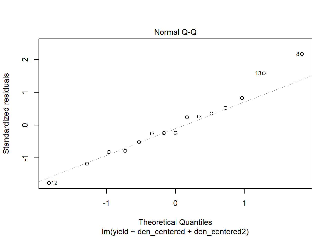
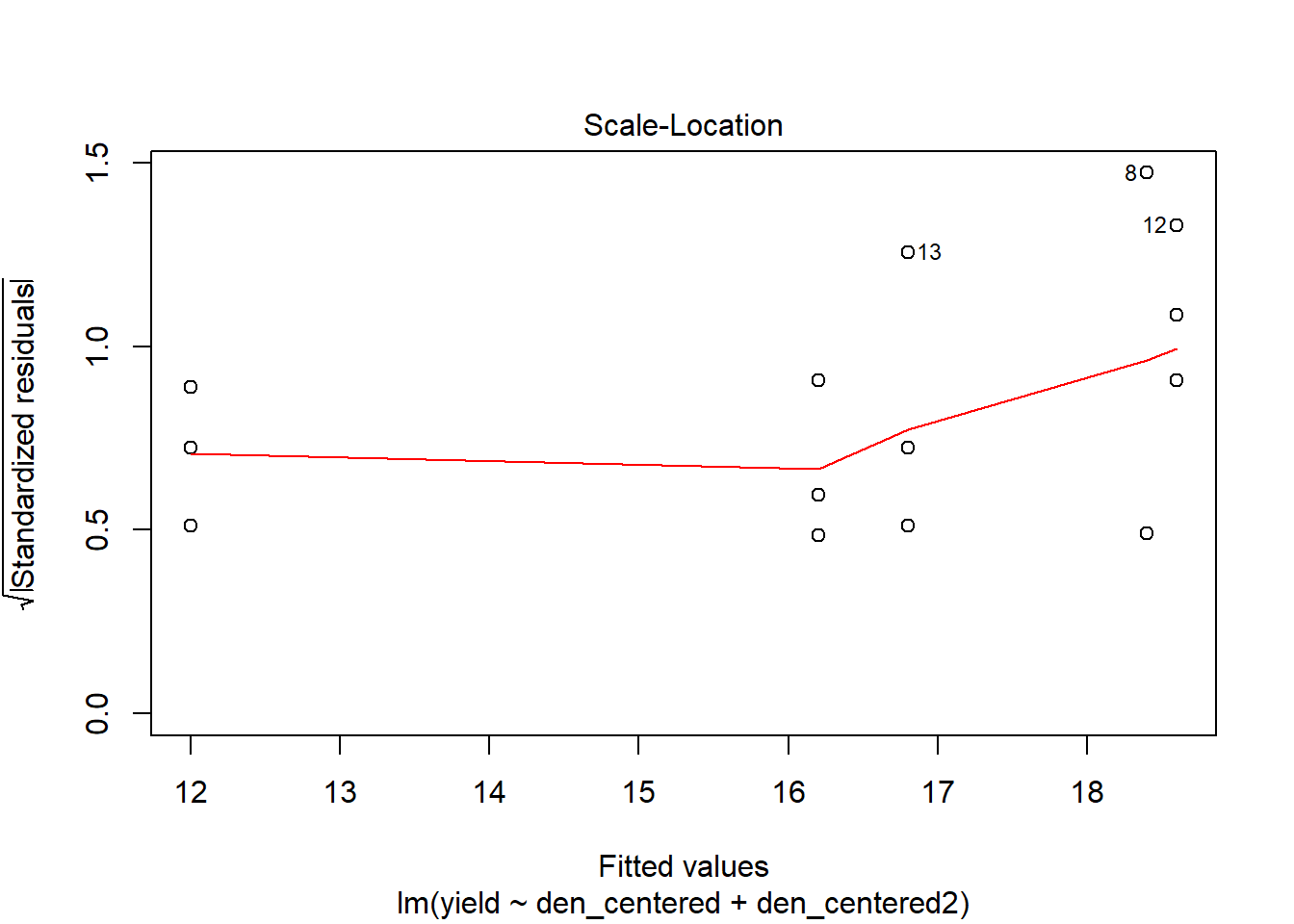
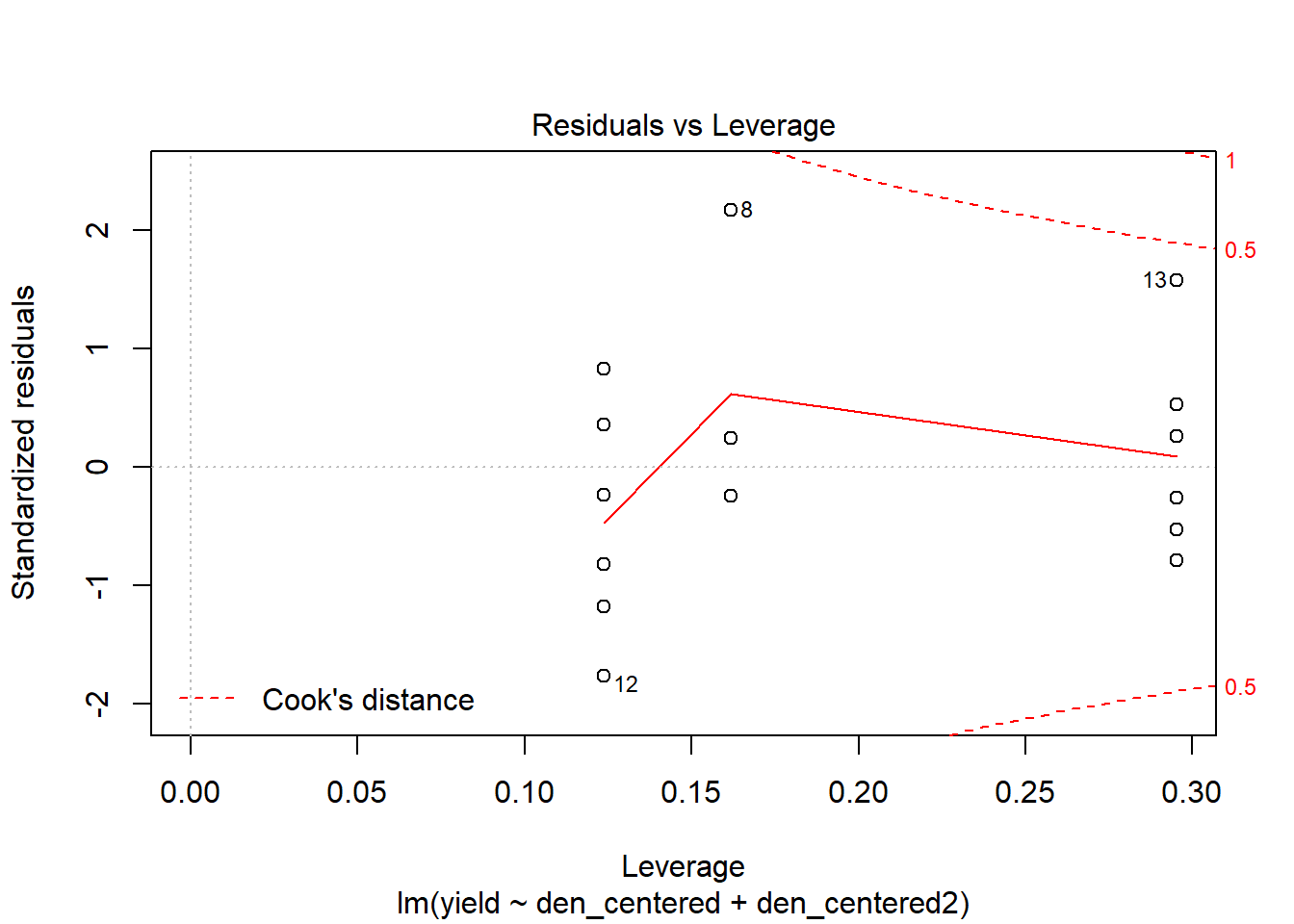
plot(model3)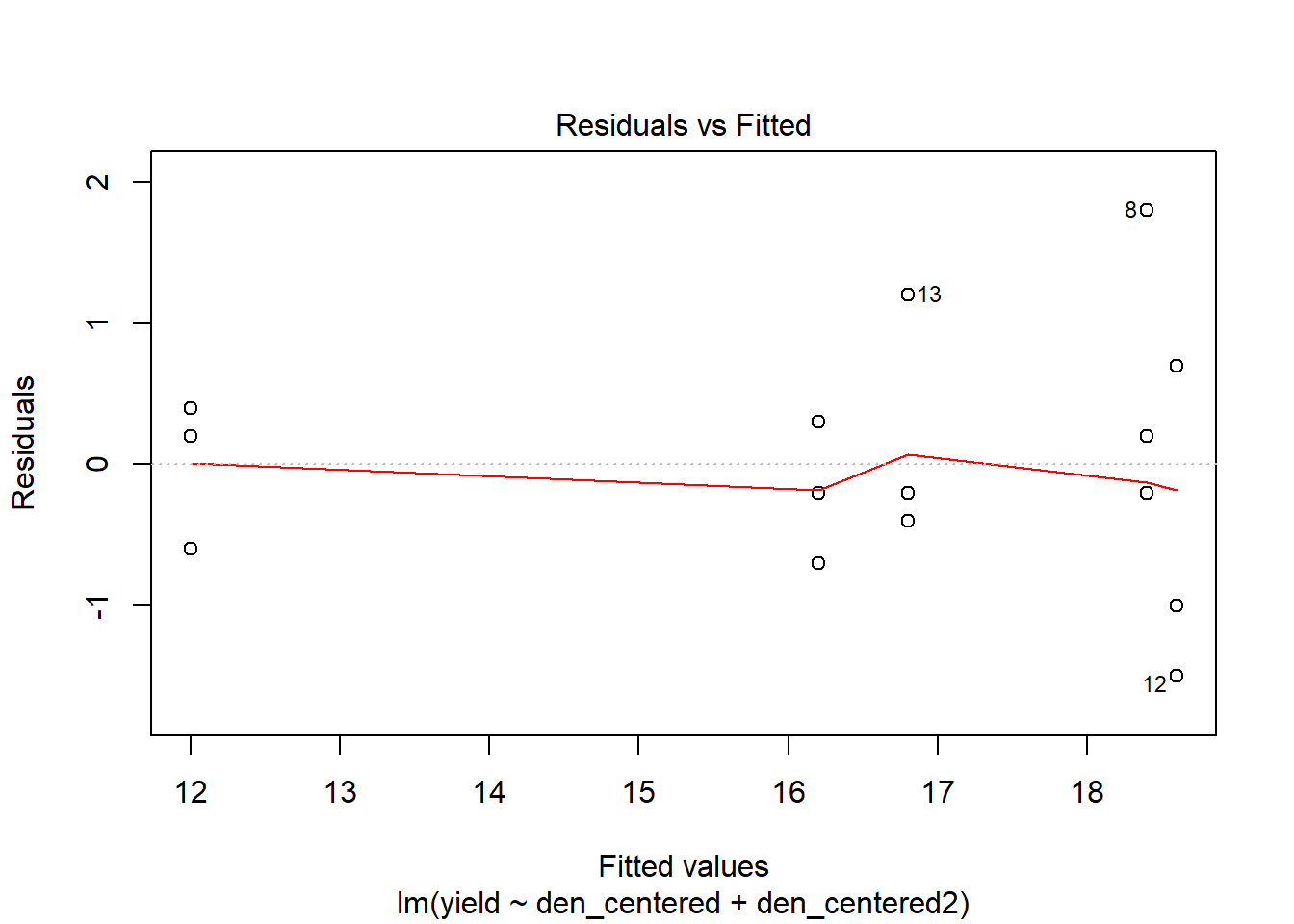
# Compare original model with the centered quadratic model
anova(model1, model3)
## Analysis of Variance Table
##
## Model 1: yield ~ density
## Model 2: yield ~ den_centered + den_centered2
## Res.Df RSS Df Sum of Sq F Pr(>F)
## 1 13 51.88
## 2 12 9.88 1 42 51.012 1.177e-05 ***
## ---
## Signif. codes: 0 '***' 0.001 '**' 0.01 '*' 0.05 '.' 0.1 ' ' 1# Collinearity?
dffits(model3)## 1 2 3 4 5 6
## 0.16317088 -0.50123382 0.32920738 -0.08494387 -0.30538465 0.12778710
## 7 8 9 10 11 12
## 0.10156307 1.16874641 -0.10156307 -0.45055886 0.30538465 -0.73883264
## 13 14 15
## 1.09610758 -0.32920738 -0.16317088dfbeta(model3)## (Intercept) den_centered den_centered2
## 1 -0.008108108 -1.891892e-03 1.351351e-04
## 2 0.024324324 5.675676e-03 -4.054054e-04
## 3 -0.016216216 -3.783784e-03 2.702703e-04
## 4 -0.026086957 7.608696e-04 5.434783e-05
## 5 -0.091304348 2.663043e-03 1.902174e-04
## 6 0.039130435 -1.141304e-03 -8.152174e-05
## 7 0.038636364 7.647245e-20 -1.136364e-04
## 8 0.347727273 9.416246e-19 -1.022727e-03
## 9 -0.038636364 1.769001e-19 1.136364e-04
## 10 -0.130434783 -3.804348e-03 2.717391e-04
## 11 0.091304348 2.663043e-03 -1.902174e-04
## 12 -0.195652174 -5.706522e-03 4.076087e-04
## 13 -0.048648649 1.135135e-02 8.108108e-04
## 14 0.016216216 -3.783784e-03 -2.702703e-04
## 15 0.008108108 -1.891892e-03 -1.351351e-04covratio(model3)## 1 2 3 4 5 6 7
## 1.8105775 1.5709359 1.7180496 1.4612786 1.2440860 1.4359881 1.5267335
## 8 9 10 11 12 13 14
## 0.3493908 1.5267335 1.0252651 1.2440860 0.6006431 0.9193090 1.7180496
## 15
## 1.8105775cooks.distance(model3)## 1 2 3 4 5 6
## 0.009626105 0.086634944 0.038504420 0.002611680 0.031993085 0.005876281
## 7 8 9 10 11 12
## 0.003732810 0.302357630 0.003732810 0.065292011 0.031993085 0.146907024
## 13 14 15
## 0.346539778 0.038504420 0.009626105vif(model3) #The value is now = 1## den_centered den_centered2
## 1 1What occurred?
We will take a look at the correlations between the original forms for density and centered forms.
cor(density, density2) #high correlation = collinearity## [1] 0.9811049cor(den_centered, den_centered2) #no correlation## [,1]
## [1,] 0Summary and considerations
The goal of this exercise was to illustrate how one needs to check any package or software regarding assumptions on linear, quadratic, higher polynomial terms. This becomes very important as you consider working with centered or standardized variables.