Background
When building a model, there are different methods we can take to construct it, ranging from manual to automated. There are strengths and weaknesses in using the different methods, but they provide a good background for those interested in taking their models to a higher level (machine level, etc.), since in those situations we are often interested to look for interactions that cannot easily be found with basic approaches.
The general idea in this example is that we are interested in examining the behaviour of the a dependent variable \(Y\) as a function of different (possible) explanatory variables, \(X_i\). The question that we are asking by looking at the different models is, “Is there a best approach to examing the different relationships?”
We will examine different approaches in this exercise and be prepared that the final model may not be the same (we will see a different example after that provides a “cleaner” model, if you will).
library(tidyverse)## -- Attaching packages ---------------------------------------------- tidyverse 1.2.1 --## v ggplot2 3.2.0 v purrr 0.3.2
## v tibble 2.1.3 v dplyr 0.8.3
## v tidyr 0.8.3 v stringr 1.4.0
## v readr 1.3.1 v forcats 0.4.0## -- Conflicts ------------------------------------------------- tidyverse_conflicts() --
## x dplyr::filter() masks stats::filter()
## x dplyr::lag() masks stats::lag()library(Hmisc)## Loading required package: lattice## Loading required package: survival## Loading required package: Formula##
## Attaching package: 'Hmisc'## The following objects are masked from 'package:dplyr':
##
## src, summarize## The following objects are masked from 'package:base':
##
## format.pval, unitslibrary(corrplot)## corrplot 0.84 loadedlibrary(readr)
library(HH)## Loading required package: grid## Loading required package: latticeExtra## Loading required package: RColorBrewer##
## Attaching package: 'latticeExtra'## The following object is masked from 'package:ggplot2':
##
## layer## Loading required package: multcomp## Loading required package: mvtnorm## Loading required package: TH.data## Loading required package: MASS##
## Attaching package: 'MASS'## The following object is masked from 'package:dplyr':
##
## select##
## Attaching package: 'TH.data'## The following object is masked from 'package:MASS':
##
## geyser## Loading required package: gridExtra##
## Attaching package: 'gridExtra'## The following object is masked from 'package:dplyr':
##
## combine##
## Attaching package: 'HH'## The following object is masked from 'package:purrr':
##
## transposelibrary(car)## Loading required package: carData##
## Attaching package: 'car'## The following objects are masked from 'package:HH':
##
## logit, vif## The following object is masked from 'package:dplyr':
##
## recode## The following object is masked from 'package:purrr':
##
## somelibrary(scatterplot3d)
library(leaps)
library(olsrr)##
## Attaching package: 'olsrr'## The following object is masked from 'package:MASS':
##
## cement## The following object is masked from 'package:datasets':
##
## riversData
For this exercise, we will examine the relationshiop between the number of aphids in 34 lots as a function of temperature and relative humidity.
lot <- c(1:34)
aphids <- c(61, 77, 87, 93, 98, 100, 104, 118, 102, 74, 63, 43, 27, 19, 14, 23, 30, 25, 67, 40, 6, 21, 18, 23, 42, 56, 60, 59, 82, 89, 77, 102, 108, 97)
temperature <- c(21, 24.8, 28.3, 26, 27.5, 27.1, 26.8, 29, 28.3, 34, 30.5, 28.3, 30.8, 31, 33.6, 31.8, 31.3, 33.5, 33, 34.5, 34.3, 34.3, 33, 26.5, 32, 27.3, 27.8, 25.8, 25, 18.5, 26, 19, 18, 16.3)
humidity <- c(57,48, 41.5, 56, 58, 31, 36.5, 41, 40, 25, 34, 13, 37, 19, 20, 17, 21, 18.5, 24.5, 16, 6, 26, 21, 26, 28, 24.5, 39, 29, 41, 53.5, 51, 48, 70, 79.5)

aphids_data <- data.frame(lot, aphids, temperature, humidity)
Basic model
Our basic model is additive, meaning we expect there to be an effect of temperature and relative humidity:
\[aphids = intercept + temperature + humidity + error\]
Our model structure will start by assuming that both temperature and humidity explain “something” about the relationship. For completeness, one could start with each factor separately and examine the explanatory value and then build the subsequent model accordingly. In many situations, what we are most interested in understanding is if there are interactions that explain better the relationships, especially if it is not clear that a linear set of assumptions is appropriate. We will build on those ideas in subsequent steps.
model_a <- with(aphids_data, lm(aphids ~ temperature + humidity))
anova(model_a) # both factors are significant
## Analysis of Variance Table
##
## Response: aphids
## Df Sum Sq Mean Sq F value Pr(>F)
## temperature 1 15194.8 15194.8 28.7765 7.554e-06 ***
## humidity 1 4813.1 4813.1 9.1151 0.005038 **
## Residuals 31 16368.9 528.0
## ---
## Signif. codes: 0 '***' 0.001 '**' 0.01 '*' 0.05 '.' 0.1 ' ' 1summary(model_a) #R^2 = 0.55##
## Call:
## lm(formula = aphids ~ temperature + humidity)
##
## Residuals:
## Min 1Q Median 3Q Max
## -35.393 -14.006 -3.198 10.335 49.265
##
## Coefficients:
## Estimate Std. Error t value Pr(>|t|)
## (Intercept) 35.8255 53.5388 0.669 0.50835
## temperature -0.6765 1.4360 -0.471 0.64089
## humidity 1.2811 0.4243 3.019 0.00504 **
## ---
## Signif. codes: 0 '***' 0.001 '**' 0.01 '*' 0.05 '.' 0.1 ' ' 1
##
## Residual standard error: 22.98 on 31 degrees of freedom
## Multiple R-squared: 0.55, Adjusted R-squared: 0.521
## F-statistic: 18.95 on 2 and 31 DF, p-value: 4.212e-06plot(model_a)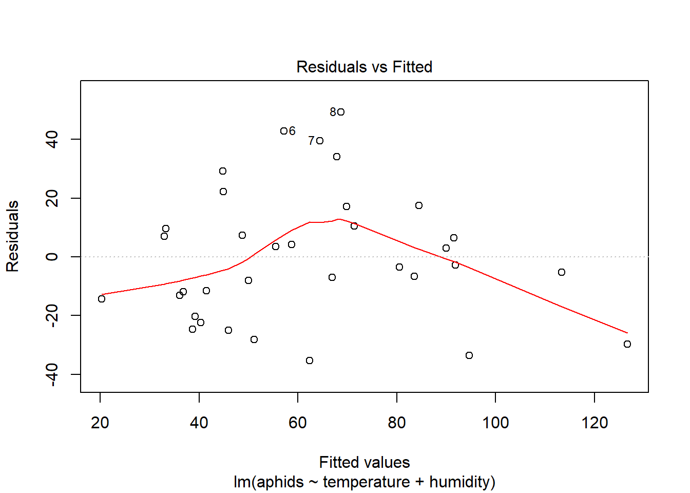
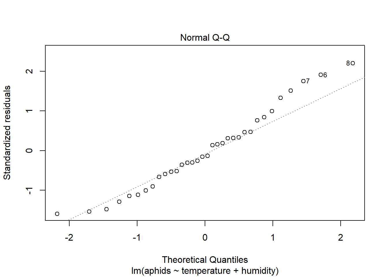
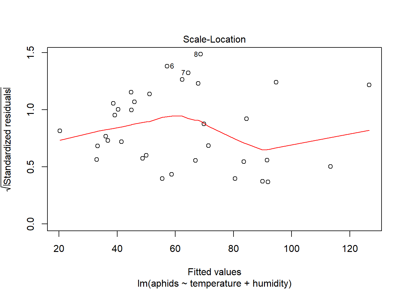
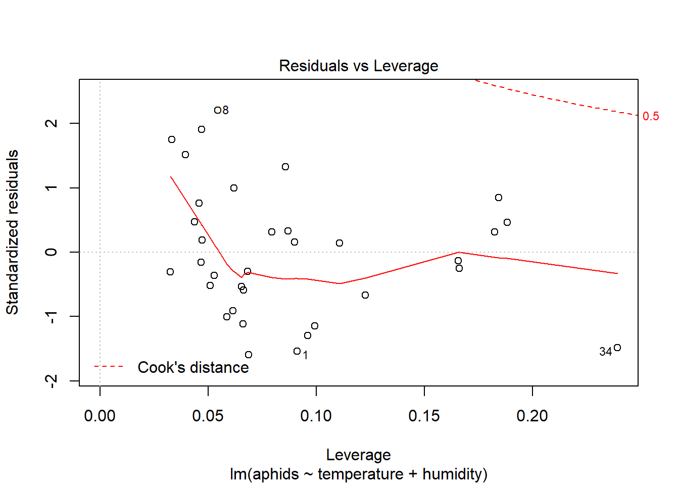
plot(model_a, which=4) 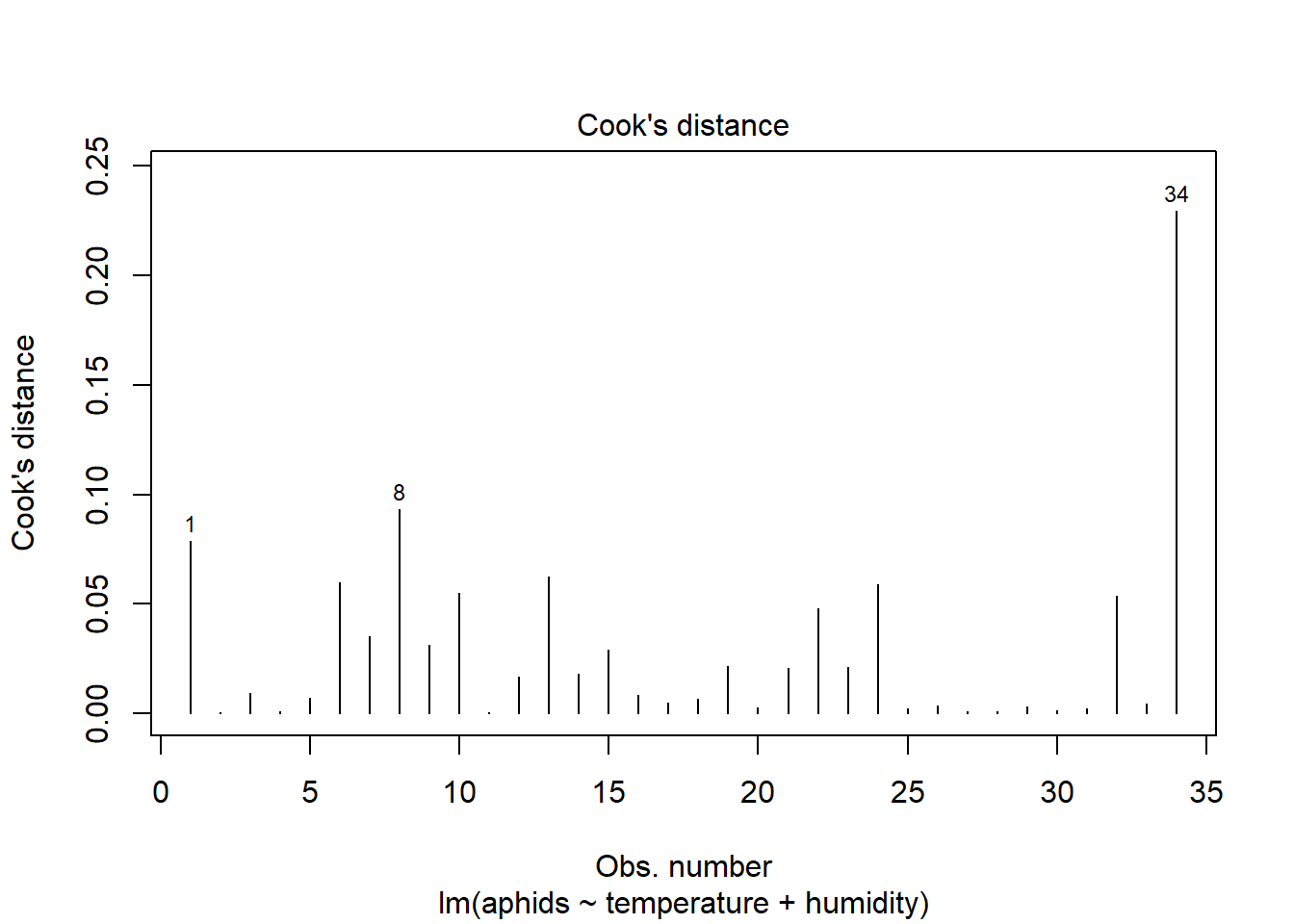
Full model
The second model we will build takes into account what we define to be the full model. In some situations, this may just be all factors and all interactions. Here, given the two potential explanatory factors and the idea that there may not be purely a linear relationship, we will build our full model based on the individual factors, the interaction between those factors, as well as a quadratic form for the model for each factor.
Model B: \(aphids = intercept + temperature + humidity + temperature^2 + humidity^2 + temperature:humidity\)
We will use an indicator function to define the quadratic model forms (\(I\)) in the subsequent model.
model_b <- with(aphids_data, lm(aphids ~ temperature + humidity + I(temperature^2) +
                                  I(humidity^2) + temperature:humidity))
anova(model_b) # significant factors: temperature, humidity, I(temperature^2)
## Analysis of Variance Table
##
## Response: aphids
## Df Sum Sq Mean Sq F value Pr(>F)
## temperature 1 15194.8 15194.8 31.4527 5.278e-06 ***
## humidity 1 4813.1 4813.1 9.9629 0.003801 **
## I(temperature^2) 1 1982.4 1982.4 4.1036 0.052418 .
## I(humidity^2) 1 805.1 805.1 1.6666 0.207279
## temperature:humidity 1 54.6 54.6 0.1129 0.739344
## Residuals 28 13526.8 483.1
## ---
## Signif. codes: 0 '***' 0.001 '**' 0.01 '*' 0.05 '.' 0.1 ' ' 1summary(model_b) #R^2 = 0.63, adjusted R^2 = 0.5617##
## Call:
## lm(formula = aphids ~ temperature + humidity + I(temperature^2) +
## I(humidity^2) + temperature:humidity)
##
## Residuals:
## Min 1Q Median 3Q Max
## -41.700 -12.220 -1.462 10.894 41.673
##
## Coefficients:
## Estimate Std. Error t value Pr(>|t|)
## (Intercept) 143.069144 610.542500 0.234 0.816
## temperature -5.639044 33.900957 -0.166 0.869
## humidity -0.182206 8.875236 -0.021 0.984
## I(temperature^2) 0.029174 0.476345 0.061 0.952
## I(humidity^2) -0.008121 0.036214 -0.224 0.824
## temperature:humidity 0.078534 0.233701 0.336 0.739
##
## Residual standard error: 21.98 on 28 degrees of freedom
## Multiple R-squared: 0.6281, Adjusted R-squared: 0.5617
## F-statistic: 9.46 on 5 and 28 DF, p-value: 2.285e-05plot(model_b)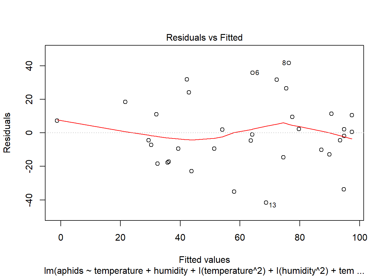
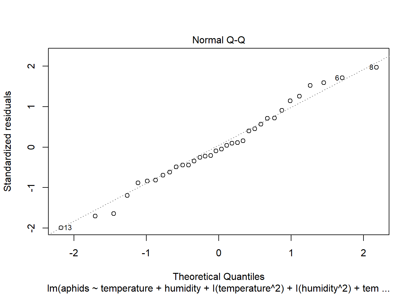
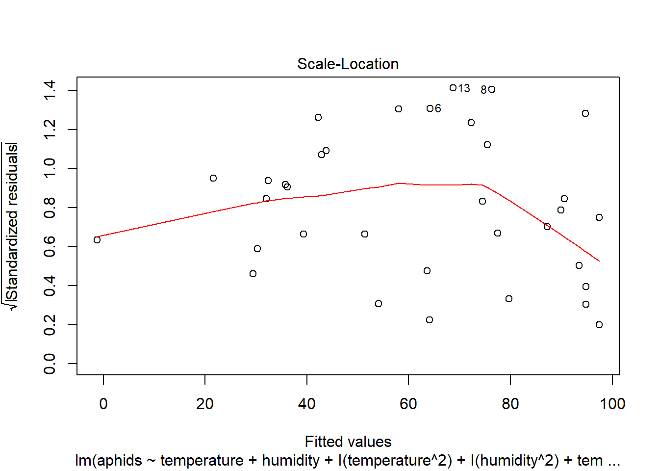
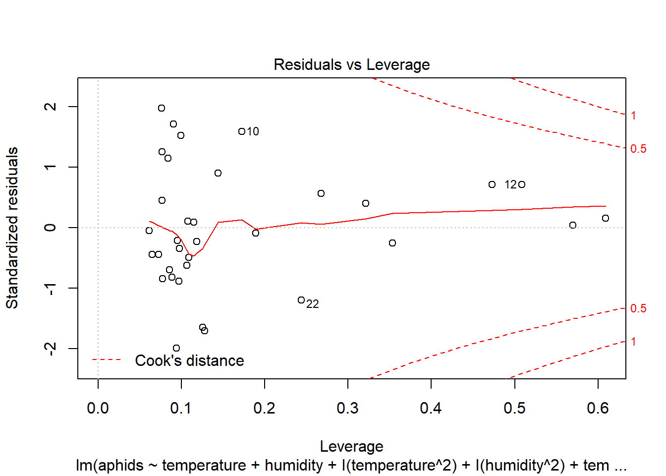
plot(model_b, which=4)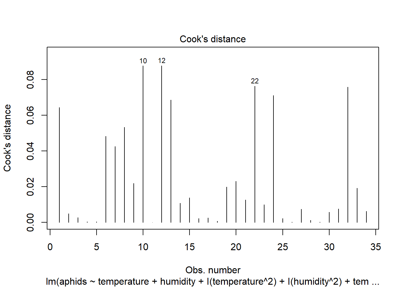
Model comparison
# anova(a,b), enables comparision between nested models, based on the number of additional parameters

anova(model_a, model_b)
## Analysis of Variance Table
##
## Model 1: aphids ~ temperature + humidity
## Model 2: aphids ~ temperature + humidity + I(temperature^2) + I(humidity^2) +
## temperature:humidity
## Res.Df RSS Df Sum of Sq F Pr(>F)
## 1 31 16369
## 2 28 13527 3 2842.1 1.961 0.1427# What the results indicates is that a full model does not explain better the relationship, probably due to being an over-adjusted model. This does not mean that they may not be a model that better explains the relationship that is less complicated. Modeling: three methods under consideration
Now, we will look at different methods to try to automate the model development. The general idea with this approach/exercise is to reduce the need to create many models and duplicate the same process over and over. The challenge will be to identify the most important factors, not just statistically, but also based on the biology and knowledge of the system.
The three methods we will consider: * Manual * Stepwise methods (“steps”) * Best subset methods
# Manual model construction
# We will start with Model B in this situation and try to reduce the complexity of the model.

# The process involves elminating factors that are not significant followed by an examination of the new model fit.

# We assume that we will work from interactions towards the simple, single factor models.

# Initial step: eliminate the factor, temperature:humidity
model_b2 <- update(model_b, .~.-temperature:humidity)
summary(model_b2)
##
## Call:
## lm(formula = aphids ~ temperature + humidity + I(temperature^2) +
## I(humidity^2))
##
## Residuals:
## Min 1Q Median 3Q Max
## -40.969 -12.837 -1.096 12.670 41.617
##
## Coefficients:
## Estimate Std. Error t value Pr(>|t|)
## (Intercept) -57.45005 127.24411 -0.451 0.6550
## temperature 5.24487 9.85861 0.532 0.5988
## humidity 2.77322 1.17389 2.362 0.0251 *
## I(temperature^2) -0.11851 0.18088 -0.655 0.5175
## I(humidity^2) -0.01921 0.01465 -1.311 0.2001
## ---
## Signif. codes: 0 '***' 0.001 '**' 0.01 '*' 0.05 '.' 0.1 ' ' 1
##
## Residual standard error: 21.64 on 29 degrees of freedom
## Multiple R-squared: 0.6266, Adjusted R-squared: 0.5752
## F-statistic: 12.17 on 4 and 29 DF, p-value: 6.302e-06anova(model_b, model_b2) ## temperature:humidity = non-significant## Analysis of Variance Table
##
## Model 1: aphids ~ temperature + humidity + I(temperature^2) + I(humidity^2) +
## temperature:humidity
## Model 2: aphids ~ temperature + humidity + I(temperature^2) + I(humidity^2)
## Res.Df RSS Df Sum of Sq F Pr(>F)
## 1 28 13527
## 2 29 13581 -1 -54.554 0.1129 0.7393# From model b2, we will now eliminate the factor I(humidity^2)
model_b3 <- update(model_b2, .~.-I(humidity^2))
summary(model_b3) # it appears that all factors explain something##
## Call:
## lm(formula = aphids ~ temperature + humidity + I(temperature^2))
##
## Residuals:
## Min 1Q Median 3Q Max
## -37.782 -13.595 -3.561 9.367 43.291
##
## Coefficients:
## Estimate Std. Error t value Pr(>|t|)
## (Intercept) -152.5753 105.7801 -1.442 0.15955
## temperature 13.9936 7.3439 1.905 0.06634 .
## humidity 1.3263 0.4050 3.275 0.00267 **
## I(temperature^2) -0.2769 0.1362 -2.033 0.05096 .
## ---
## Signif. codes: 0 '***' 0.001 '**' 0.01 '*' 0.05 '.' 0.1 ' ' 1
##
## Residual standard error: 21.9 on 30 degrees of freedom
## Multiple R-squared: 0.6045, Adjusted R-squared: 0.565
## F-statistic: 15.29 on 3 and 30 DF, p-value: 3.217e-06# Compare the models b2 and b3
anova(model_b2, model_b3) # I(humidity^2) = not signficant ## Analysis of Variance Table
##
## Model 1: aphids ~ temperature + humidity + I(temperature^2) + I(humidity^2)
## Model 2: aphids ~ temperature + humidity + I(temperature^2)
## Res.Df RSS Df Sum of Sq F Pr(>F)
## 1 29 13581
## 2 30 14386 -1 -805.11 1.7191 0.2001# Compare with baseline model
anova(model_a, model_b3) ## this model is close to p=0,05 and probably has ## Analysis of Variance Table
##
## Model 1: aphids ~ temperature + humidity
## Model 2: aphids ~ temperature + humidity + I(temperature^2)
## Res.Df RSS Df Sum of Sq F Pr(>F)
## 1 31 16369
## 2 30 14386 1 1982.4 4.1339 0.05096 .
## ---
## Signif. codes: 0 '***' 0.001 '**' 0.01 '*' 0.05 '.' 0.1 ' ' 1# some predictive value
# From model b2 (no interaction), we will now remove temperature to
# look at the humidity^2 term
model_b3t <- update(model_b2, .~.-I(temperature^2))
summary(model_b3t) # it appears that all factors explain something##
## Call:
## lm(formula = aphids ~ temperature + humidity + I(humidity^2))
##
## Residuals:
## Min 1Q Median 3Q Max
## -41.466 -10.864 -0.372 9.754 42.475
##
## Coefficients:
## Estimate Std. Error t value Pr(>|t|)
## (Intercept) 18.95111 50.44302 0.376 0.70979
## temperature -1.15206 1.35435 -0.851 0.40171
## humidity 3.24552 0.91764 3.537 0.00134 **
## I(humidity^2) -0.02563 0.01080 -2.373 0.02426 *
## ---
## Signif. codes: 0 '***' 0.001 '**' 0.01 '*' 0.05 '.' 0.1 ' ' 1
##
## Residual standard error: 21.43 on 30 degrees of freedom
## Multiple R-squared: 0.6211, Adjusted R-squared: 0.5832
## F-statistic: 16.39 on 3 and 30 DF, p-value: 1.711e-06anova(model_a, model_b3t)## Analysis of Variance Table
##
## Model 1: aphids ~ temperature + humidity
## Model 2: aphids ~ temperature + humidity + I(humidity^2)
## Res.Df RSS Df Sum of Sq F Pr(>F)
## 1 31 16369
## 2 30 13782 1 2586.5 5.63 0.02426 *
## ---
## Signif. codes: 0 '***' 0.001 '**' 0.01 '*' 0.05 '.' 0.1 ' ' 1anova(model_b2, model_b3t)## Analysis of Variance Table
##
## Model 1: aphids ~ temperature + humidity + I(temperature^2) + I(humidity^2)
## Model 2: aphids ~ temperature + humidity + I(humidity^2)
## Res.Df RSS Df Sum of Sq F Pr(>F)
## 1 29 13581
## 2 30 13782 -1 -201.05 0.4293 0.5175# From model b3, remove temperature^2 (can do the same with model_b3t)
model_b4 <- update(model_b3, .~.-I(temperature^2))
anova(model_b4)## Analysis of Variance Table
##
## Response: aphids
## Df Sum Sq Mean Sq F value Pr(>F)
## temperature 1 15194.8 15194.8 28.7765 7.554e-06 ***
## humidity 1 4813.1 4813.1 9.1151 0.005038 **
## Residuals 31 16368.9 528.0
## ---
## Signif. codes: 0 '***' 0.001 '**' 0.01 '*' 0.05 '.' 0.1 ' ' 1summary(model_b4)##
## Call:
## lm(formula = aphids ~ temperature + humidity)
##
## Residuals:
## Min 1Q Median 3Q Max
## -35.393 -14.006 -3.198 10.335 49.265
##
## Coefficients:
## Estimate Std. Error t value Pr(>|t|)
## (Intercept) 35.8255 53.5388 0.669 0.50835
## temperature -0.6765 1.4360 -0.471 0.64089
## humidity 1.2811 0.4243 3.019 0.00504 **
## ---
## Signif. codes: 0 '***' 0.001 '**' 0.01 '*' 0.05 '.' 0.1 ' ' 1
##
## Residual standard error: 22.98 on 31 degrees of freedom
## Multiple R-squared: 0.55, Adjusted R-squared: 0.521
## F-statistic: 18.95 on 2 and 31 DF, p-value: 4.212e-06anova(model_b3, model_b4) ## Analysis of Variance Table
##
## Model 1: aphids ~ temperature + humidity + I(temperature^2)
## Model 2: aphids ~ temperature + humidity
## Res.Df RSS Df Sum of Sq F Pr(>F)
## 1 30 14386
## 2 31 16369 -1 -1982.4 4.1339 0.05096 .
## ---
## Signif. codes: 0 '***' 0.001 '**' 0.01 '*' 0.05 '.' 0.1 ' ' 1# You can continue reducing the model, but we do know now that there is some predictive value with the variables we have Stepwise methods
Now, let’s use the function step() to automate the search process for the best model.
What is required typically is the definition of the null model and the full model. With these defined, we can use “forward”, “backward”, or “both” direction searching.
## Stepwise methods

# Null model
model_null <- lm(aphids~1, data=aphids_data)
model_full <- model_b

# Forward
forward <- step(model_null, scope=list(lower=model_null, upper=model_full,
                                       direction="forward"))
## Start: AIC=239.16
## aphids ~ 1
##
## Df Sum of Sq RSS AIC
## + humidity 1 19891 16486 214.25
## + I(temperature^2) 1 16098 20279 221.29
## + I(humidity^2) 1 15560 20817 222.18
## + temperature 1 15195 21182 222.77
## <none> 36377 239.16
##
## Step: AIC=214.25
## aphids ~ humidity
##
## Df Sum of Sq RSS AIC
## + I(humidity^2) 1 2371.2 14115 210.97
## <none> 16486 214.25
## + I(temperature^2) 1 358.4 16128 215.51
## + temperature 1 117.2 16369 216.01
## - humidity 1 19890.7 36377 239.16
##
## Step: AIC=210.97
## aphids ~ humidity + I(humidity^2)
##
## Df Sum of Sq RSS AIC
## <none> 14115 210.97
## + I(temperature^2) 1 400.9 13714 211.99
## + temperature 1 332.4 13782 212.16
## - I(humidity^2) 1 2371.2 16486 214.25
## - humidity 1 6702.0 20817 222.18# Backwards
back <- step(model_null, scope=list(lower=model_null, upper=model_full,
direction="backward")) ## Start: AIC=239.16
## aphids ~ 1
##
## Df Sum of Sq RSS AIC
## + humidity 1 19891 16486 214.25
## + I(temperature^2) 1 16098 20279 221.29
## + I(humidity^2) 1 15560 20817 222.18
## + temperature 1 15195 21182 222.77
## <none> 36377 239.16
##
## Step: AIC=214.25
## aphids ~ humidity
##
## Df Sum of Sq RSS AIC
## + I(humidity^2) 1 2371.2 14115 210.97
## <none> 16486 214.25
## + I(temperature^2) 1 358.4 16128 215.51
## + temperature 1 117.2 16369 216.01
## - humidity 1 19890.7 36377 239.16
##
## Step: AIC=210.97
## aphids ~ humidity + I(humidity^2)
##
## Df Sum of Sq RSS AIC
## <none> 14115 210.97
## + I(temperature^2) 1 400.9 13714 211.99
## + temperature 1 332.4 13782 212.16
## - I(humidity^2) 1 2371.2 16486 214.25
## - humidity 1 6702.0 20817 222.18# Both directions
back <- step(model_null, scope=list(lower=model_null, upper=model_full,
direction="both"))## Start: AIC=239.16
## aphids ~ 1
##
## Df Sum of Sq RSS AIC
## + humidity 1 19891 16486 214.25
## + I(temperature^2) 1 16098 20279 221.29
## + I(humidity^2) 1 15560 20817 222.18
## + temperature 1 15195 21182 222.77
## <none> 36377 239.16
##
## Step: AIC=214.25
## aphids ~ humidity
##
## Df Sum of Sq RSS AIC
## + I(humidity^2) 1 2371.2 14115 210.97
## <none> 16486 214.25
## + I(temperature^2) 1 358.4 16128 215.51
## + temperature 1 117.2 16369 216.01
## - humidity 1 19890.7 36377 239.16
##
## Step: AIC=210.97
## aphids ~ humidity + I(humidity^2)
##
## Df Sum of Sq RSS AIC
## <none> 14115 210.97
## + I(temperature^2) 1 400.9 13714 211.99
## + temperature 1 332.4 13782 212.16
## - I(humidity^2) 1 2371.2 16486 214.25
## - humidity 1 6702.0 20817 222.18Return to manual model
For the moment, let’s return to our manual model to take a look at suggest model from the stepwise procedure.
model_b5<-with(aphids_data, lm(aphids~humidity+I(humidity^2)))
anova(model_b5)
## Analysis of Variance Table
##
## Response: aphids
## Df Sum Sq Mean Sq F value Pr(>F)
## humidity 1 19890.7 19890.7 43.6854 2.194e-07 ***
## I(humidity^2) 1 2371.2 2371.2 5.2079 0.0295 *
## Residuals 31 14114.8 455.3
## ---
## Signif. codes: 0 '***' 0.001 '**' 0.01 '*' 0.05 '.' 0.1 ' ' 1summary(model_b5)##
## Call:
## lm(formula = aphids ~ humidity + I(humidity^2))
##
## Residuals:
## Min 1Q Median 3Q Max
## -44.703 -13.018 -0.288 12.098 40.196
##
## Coefficients:
## Estimate Std. Error t value Pr(>|t|)
## (Intercept) -21.54288 16.60909 -1.297 0.204184
## humidity 3.41812 0.89093 3.837 0.000574 ***
## I(humidity^2) -0.02427 0.01063 -2.282 0.029504 *
## ---
## Signif. codes: 0 '***' 0.001 '**' 0.01 '*' 0.05 '.' 0.1 ' ' 1
##
## Residual standard error: 21.34 on 31 degrees of freedom
## Multiple R-squared: 0.612, Adjusted R-squared: 0.5869
## F-statistic: 24.45 on 2 and 31 DF, p-value: 4.238e-07Best subsets
In the last section of this exercise, we will use a method based on best subsets regression. We will use the funtion regsubsets in the package leaps to do this exercise. This method looks at the full model and considers different combinations of models based on the number of best models we decide to examine. The result is not necessarily what is the best model but rather a series of models that explain something in our model. We would then need to go back, after model selection, and run the formal analysis to look at model fit, predictive value, biological relevance, etc..
# regsubsets = package *leaps*

# let's start by looking at the best 3 models per level
subsets <- regsubsets(aphids~temperature+humidity+I(temperature^2)+
I(humidity^2)+temperature:humidity, nbest=3, data=aphids_data)

plot(subsets, scale="adjr2")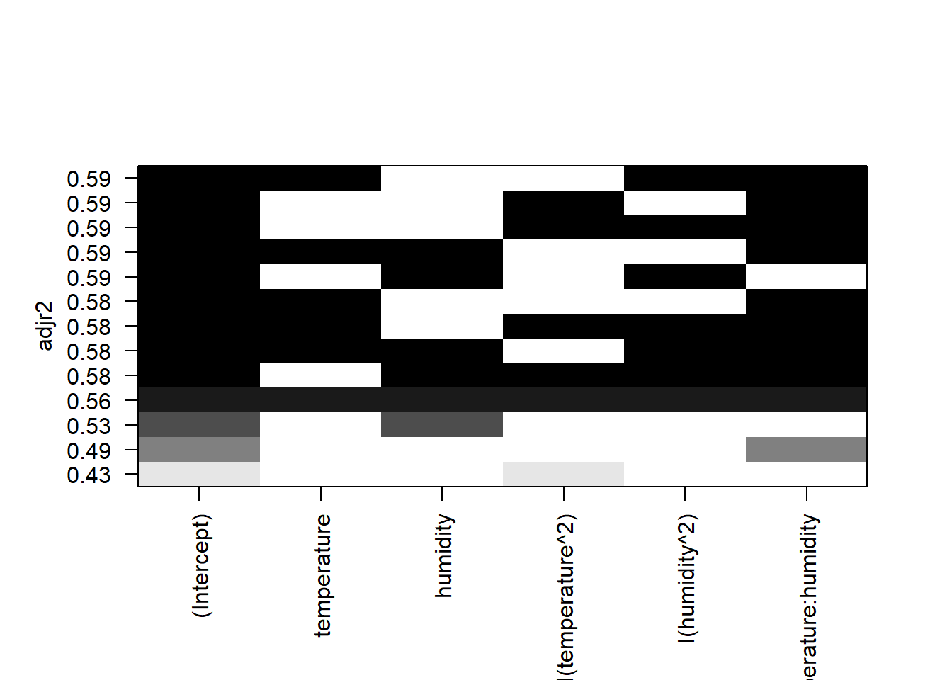
plot(subsets, scale="bic")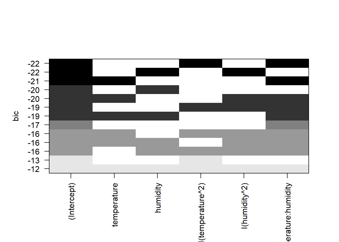
plot(subsets, scale="Cp")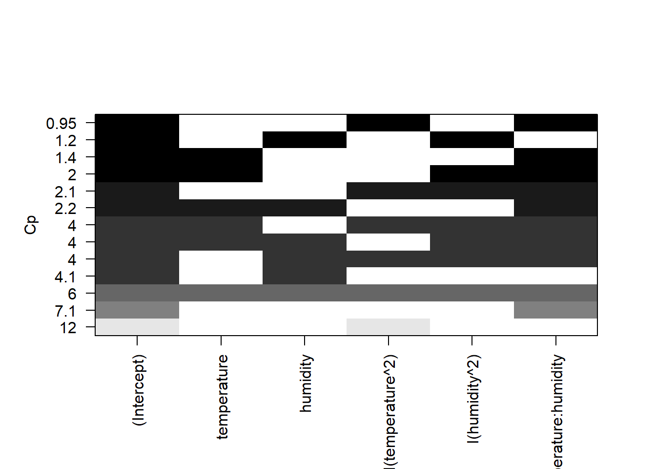
Summary
Hopefully you saw that this was not an easy exercise since there was not a clear model that best fit the response. In modeling we are integrating mathematical/statistical concepts with computational methodology, as well as keeping in mind the biology/pathology.
What is the best method to model observaed relationships?
For this concluding part, I draw and adapt on ideas from Gelman and Hall (2007; Data Analysis Using Regression and Multilevel/Hierarchical Models):
- Include all variables that for reasons known to the researcher may be important for predicting an outcome.
- You do not always have to include all inputs as separate predictors. You can consider in some situations that several inputs could be averaged or summed to create a “total score” that then becomes the predictor variable (index value, etc.)
- For predictive variables with large effects, an examination of the interactions may also be warranted (very common when we extend this to regression trees and other methods).
- Strategy for decisions focused on excluding a variable based on the expected sign and statistical significance:
- If the predictor is not statistically significant and has the expected sign (+ or -), in general it is fine to keep the predictor. This means that while the predictor is not helping predictions dramatically, it is also not hurting them.
- If the predictor is not statistically significant and does not have the expected sign, consider removing this from the model (i.e., the coefficiente is set to 0).
- If the predictor is statistically significant but does not have the expected sign, this is somewhat more complicated since the challenge is in terms of interpretation. Consider trying to gather additional data on lurking variables and include those in the analysis.
- If the predictor is statistically significant and has the expected sign, definitely you should keep this in the model!